Table 2: Chi-squared test between Sex and FC groups.
Pearson’s Chi-squared test: demo$Sex and demo$cat
Test statistic
df
P value
14.2
2
0.0008269 * * *
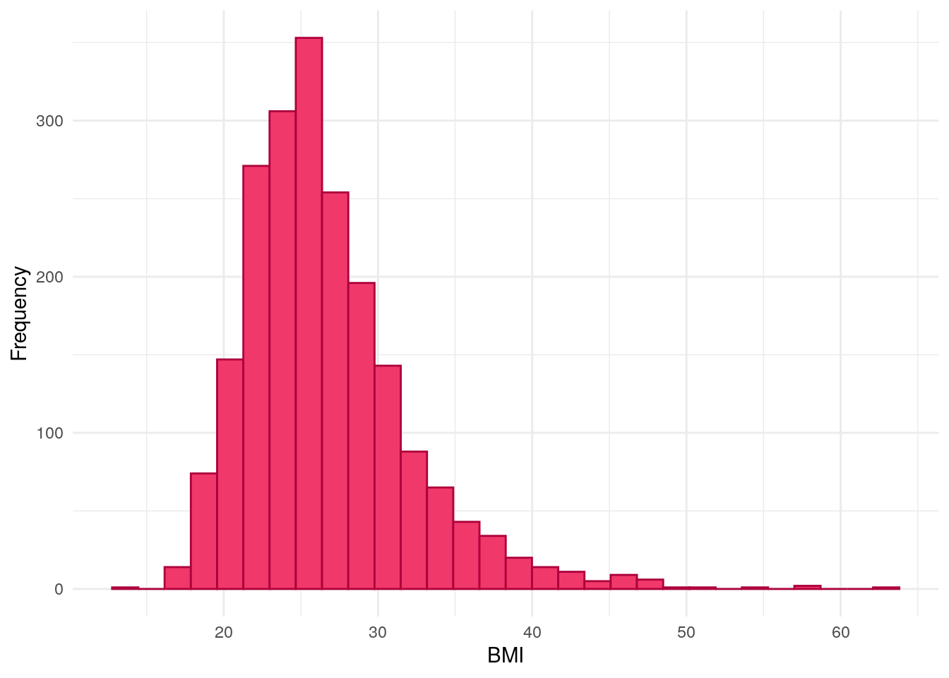
BMI
Body mass index is given by weight (in Kg) divided by height (in M) squared.
As thresholds differ in the paediatric population, and are dependent on both age and sex, BMI has not been calculated for those less than 18 years of age. BMI is first considered as a continuous variable.
Table 3: Fisher’s exact test between BMI and FC groups.
Analysis of Variance Model
Df
Sum Sq
Mean Sq
F value
Pr(>F)
cat
2
134.9
67.45
2.387
0.09219
Residuals
2057
58135
28.26
NA
NA
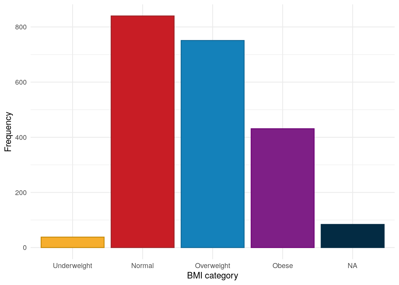
We also consider BMI grouped into underweight, normal, overweight, and obese categories using the definitions used by the NIH and WHO (Weir and Jan 2024).
A cut-off of 30 KgM^{-2} is used to denote obesity in adults without Asian/South Asian backgrounds. As data on Asian and South Asian ethnicity is not available (See Ethnicity), we are unable to adjust the threshold based on ethnicity. However, this is expected to be relevant to relatively few subjects.
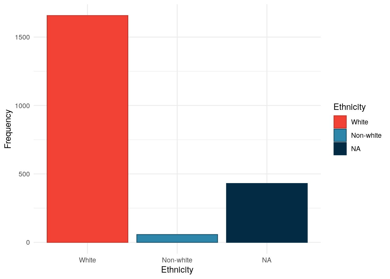
Table 5: Chi-squared test between ethnicity and FC groups.
Pearson’s Chi-squared test: demo$Ethnicity and demo$cat
Test statistic
df
P value
2.416
2
0.2989
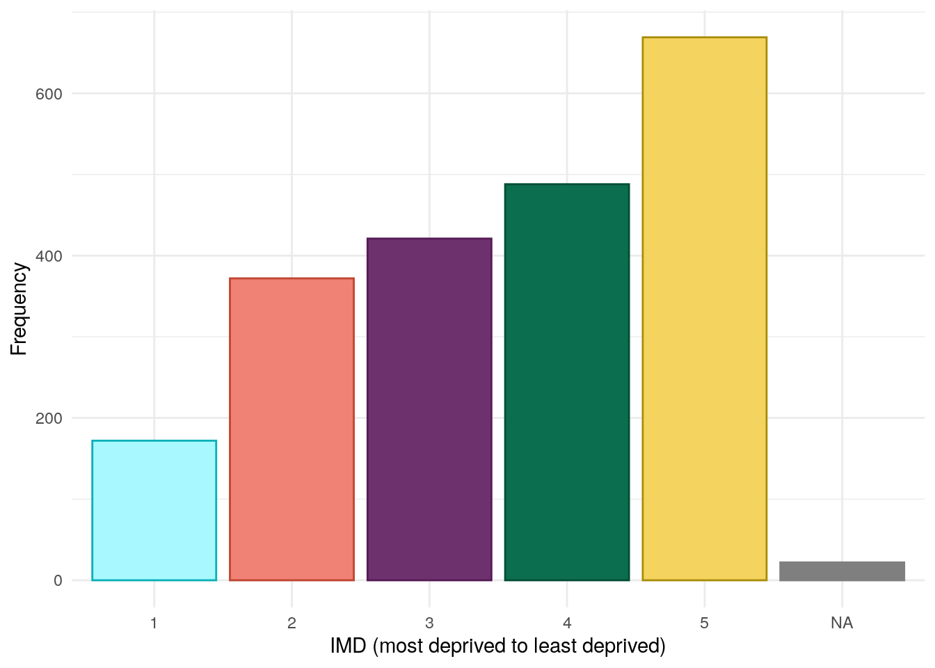
Index of multiple deprivation
The PREdiCCt SAP states the primary analyses will be controlled for by index of multiple deprivation (IMD). It should be noted that the PREdiCCt study recruited across the UK and there is no consistent measure of IMD across the whole of the UK. Instead, IMD measures are handled slightly differently by each constituent nation.
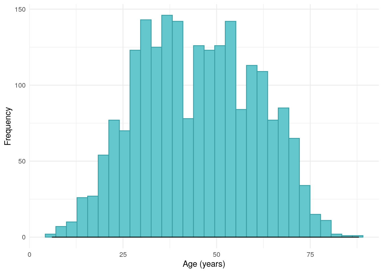
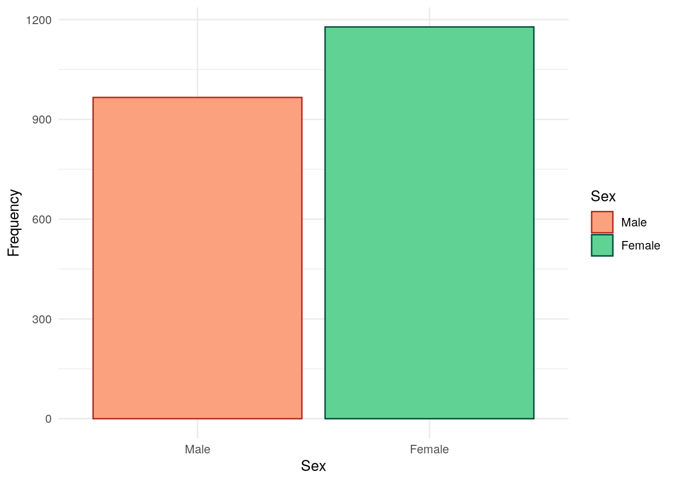
---title: "Demographic data"author: - name: "Nathan Constantine-Cooke" corresponding: true url: https://scholar.google.com/citations?user=2emHWR0AAAAJ&hl=en&oi=ao affiliations: - ref: IGCbibliography: Baseline.bib ---## Introduction```{R}set.seed(123)source("Baseline/utils.R")################ Packages ################library(plyr) # Used for mapping valuessuppressPackageStartupMessages(library(tidyverse)) # ggplot2, dplyr, and magrittrlibrary(readxl) # Read in Excel fileslibrary(lubridate) # Handle dateslibrary(datefixR) # Standardise dateslibrary(patchwork) # Arrange ggplots# Generate tablessuppressPackageStartupMessages(library(table1))library(knitr)library(pander)# Generate flowchart of cohort derivationlibrary(DiagrammeR)library(DiagrammeRsvg)# paths to PREdiCCt dataif (file.exists("/docker")) { # If running in docker data.path <-"data/final/20221004/" redcap.path <-"data/final/20231030/" prefix <-"data/end-of-follow-up/" outdir <-"data/processed/"} else { # Run on OS directly data.path <-"/Volumes/igmm/cvallejo-predicct/predicct/final/20221004/" redcap.path <-"/Volumes/igmm/cvallejo-predicct/predicct/final/20231030/" prefix <-"/Volumes/igmm/cvallejo-predicct/predicct/end-of-follow-up/" outdir <-"/Volumes/igmm/cvallejo-predicct/predicct/processed/"}demo <-read_xlsx(paste0(data.path, "Baseline2022/demographics.xlsx"),col_types =c("text","text","text","text","numeric","numeric","text","text","date","numeric","text" ))fcal <-read_xlsx(paste0(data.path, "Baseline2022/calprotectin.xlsx"))fcal$Result <-as.numeric(plyr::mapvalues(fcal$Result, from ="<20", to =20))fcal <- fcal[, c("ParticipantNo", "Result")]fcal.eof <-read_xlsx(paste0(prefix, "EOF_fcal.xlsx"))fcal.eof <-subset(fcal.eof, IsBaseline ==1)fcal.eof <-subset(fcal.eof, FCALLevel !=".")fcal.eof$FCALLevel <-as.numeric(fcal.eof$FCALLevel)fcal.eof <- fcal.eof[, c("ParticipantNo", "FCALLevel")]names(fcal.eof)[2] <-"Result"fcal <-rbind(fcal, fcal.eof)fcal <-distinct(fcal, ParticipantNo, .keep_all =TRUE)fcal$cat <-0for (i in1:nrow(fcal)) {if (fcal[i, "Result"] <50) fcal[i, "cat"] <-1if ((fcal[i, "Result"] >=50) & (fcal[i, "Result"] <=250)) fcal[i, "cat"] <-2if (fcal[i, "Result"] >250) fcal[i, "cat"] <-3}demo <-merge(demo, fcal[, c("ParticipantNo", "Result", "cat")],by ="ParticipantNo",all.x =TRUE,all.y =FALSE)demo$cat <-factor(demo$cat,levels =c(1, 2, 3),labels =c("FC < 50", "FC 50-250", "FC > 250"))names(demo)[12] <-"FC"# Result ~> FC```This page describes key demographic data collected by the PREdiCCt study.## AgeThe distribution of age for the study cohort is approximately normallydistributed. ```{R}#| label: fig-age-dist#| fig-cap: "Distribution of age in the FC cohort."demo %>%drop_na(cat) %>%ggplot(aes(x = age)) +geom_histogram(bins =30, fill ="#64c7ce", color ="#3B9EA4") +geom_density() +theme_minimal() +xlab("Age (years)") +ylab("Frequency")```Age is significantly associated with faecal calprotectin. ```{R}#| label: tbl-age-fc#| tbl-cap: "ANOVA between age and FC groups."pander(summary(aov(age ~ cat, data = demo)))```## SexSex was self-reported via subject questionnaires. As can be seen in@fig-sex-dist, the PREdiCCt cohort is female by majority. ```{R}#| label: fig-sex-dist#| fig-cap: "Distribution of sex in the FC cohort."demo$Sex <-factor(demo$Sex, levels =c("1", "2"), labels =c("Male", "Female"))demo %>%drop_na(cat) %>%ggplot(aes(x = Sex, fill = Sex, color = Sex)) +geom_bar() +ylab("Frequency") +theme_minimal() +scale_fill_manual(values =c("#FCA17D", "#60D394")) +scale_color_manual(values =c("#B22A21", "#034C3C"))```Moreover, the distribution of sex is significantly different between FCAL groups. ```{R}#| label: tbl-sex-fc#| tbl-cap: "Chi-squared test between Sex and FC groups."pander(chisq.test(demo$Sex, demo$cat))```## BMIBody mass index is given by weight (in $Kg$) divided by height (in $M$) squared.As thresholds differ in the paediatric population, and are dependent on both ageand sex, BMI has not been calculated for those less than 18 years of age. BMI isfirst considered as a continuous variable. ```{R}#| label: fig-BMI-dist#| fig-cap: "Distribution of BMI in the FC cohort."#| warning: falsedemo$BMI <-with(demo, Weight / ((Height /100)^2))demo[demo[, "age"] <18, "BMI"] <-NAp <- demo %>%ggplot(aes(x = BMI)) +geom_histogram(color ="#AD013B", fill ="#F0386B", bins =30) +theme_minimal(base_family ="sans") +ylab("Frequency")ggsave("plots/BMI-full-cohort.png", p,width =9,height =6)ggsave("plots/BMI-full-cohort.pdf", p, width =9, height =6)demo %>%drop_na(cat) %>%ggplot(aes(x = BMI)) +geom_histogram(color ="#AD013B", fill ="#F0386B", bins =30) +theme_minimal() +ylab("Frequency")```BMI as a continuous variable is not associated with FC groups. ```{R}#| label: tbl-BMI-fc#| tbl-cap: "Fisher's exact test between BMI and FC groups."pander(summary(aov(BMI ~ cat, data = demo)))```We also consider BMI grouped into underweight, normal, overweight, and obesecategories using the definitions used by the NIH and WHO[@weirBMIClassificationPercentile2024]. A cut-off of $30 KgM^{-2}$ is used to denote obesity in adults withoutAsian/South Asian backgrounds. As data on Asian and South Asian ethnicity is notavailable (See [Ethnicity](#ethnicity)), we are unable to adjust the thresholdbased on ethnicity. However, this is expected to be relevant to relatively fewsubjects.```{R}#| label: fig-BMIcat-dist#| fig-cap: "Distribution of BMI categories in the FC cohort."demo$BMIcat <-cut(demo$BMI,c(0, 18.5, 25, 30, Inf),include.lowest =TRUE,right =FALSE,labels =c("Underweight", "Normal", "Overweight", "Obese"))demo[demo[, "age"] <18, "BMIcat"] <-NAplt.cols <-c("#F6AE2D", "#C81D25", "#1481BA", "#7E1F86")demo %>%drop_na(cat) %>%ggplot(aes(x = BMIcat, color = BMIcat, fill = BMIcat)) +geom_bar() +theme_minimal() +theme(legend.position ="none") +scale_fill_manual(values = plt.cols, na.value ="#032B43") +scale_color_manual(values = colorspace::darken(plt.cols, 0.2),na.value ="#032B43" ) +xlab("BMI category") +ylab("Frequency")```BMI by category is not associated with FC groups. ```{R}#| label: tbl-BMIcat-fc#| tbl-cap: "Chi-squared test between BMI categories and FC groups."pander(chisq.test(demo$BMIcat, demo$cat))```## EthnicityDue to low counts for non-white ethnicities, we are only able to reportfrequencies of white and non-white ethnicities. ```{R}#| label: fig-ethnic-dist#| fig-cap: "Distribution of ethnicity in the FC cohort."demo$ethnic_gp <-factor(demo$ethnic_gp,levels =c("1", "2"),labels =c("White", "Non-white"))colnames(demo)[10:11] <-c("Age", "Ethnicity")demo %>%drop_na(cat) %>%ggplot(aes(x = Ethnicity, fill = Ethnicity, color = Ethnicity)) +geom_bar() +ylab("Frequency") +theme_minimal() +scale_fill_manual(values =c("#F24236", "#2E86AB"), na.value ="#032B43") +scale_color_manual(values =c("#C0362C", "#1E556C"), na.value ="#032B43")``````{R}#| label: tbl-ethnicity-fc#| tbl-cap: "Chi-squared test between ethnicity and FC groups."pander(chisq.test(demo$Ethnicity, demo$cat))```## Index of multiple deprivationThe PREdiCCt SAP states the primary analyses will be controlled for by indexof multiple deprivation (IMD). It should be noted that the PREdiCCt studyrecruited across the UK and there is no consistent measure of IMD across thewhole of the UK. Instead, IMD measures are handled slightly differently by each constituent nation. ```{R}#| label: fig-imd-dist#| fig-cap: "Distribution of IMD."#| warning: falseIMD <-read_xlsx(paste0(redcap.path, "/IMD.xlsx"))IMD <-as.data.frame(IMD)names(IMD)[2] <-"IMD"demo <-merge(demo, IMD, by ="ParticipantNo", all.x =TRUE, all.y =FALSE)demo$IMD <-as.factor(demo$IMD)cols <-c("#A8F9FF", "#EF8275", "#6D326D", "#0B6E4F", "#F4D35E")demo %>%drop_na(cat) %>%ggplot(aes(x = IMD, color =as.factor(IMD), fill =as.factor(IMD))) +geom_bar() +theme_minimal() +theme(legend.position ="none") +ylab("Frequency") +xlab("IMD (most deprived to least deprived)") +scale_fill_manual(values = cols) +scale_color_manual(values = colorspace::darken(cols, amount =0.3))``````{R}#| label: tbl-IMD-fc#| tbl-cap: "CHI-squared test between IMD and FC groups."pander(chisq.test(demo$IMD, demo$cat))```## Missingness```{R}demo %>%select( Age, Sex, BMI, IMD, SiteName ) %>%missing_plot2(title ="Demographics missingness")``````{R}saveRDS(demo, paste0(outdir, "demo-demographics.RDS"))```## Reproduction and reproducibility {.appendix}<details class = "appendix"> <summary> Session info </summary>```{R Session info}#| echo: falsepander::pander(sessionInfo())```</details>Licensed by <a href="https://creativecommons.org/licenses/by/4.0/">CC BY</a> unless otherwise stated.