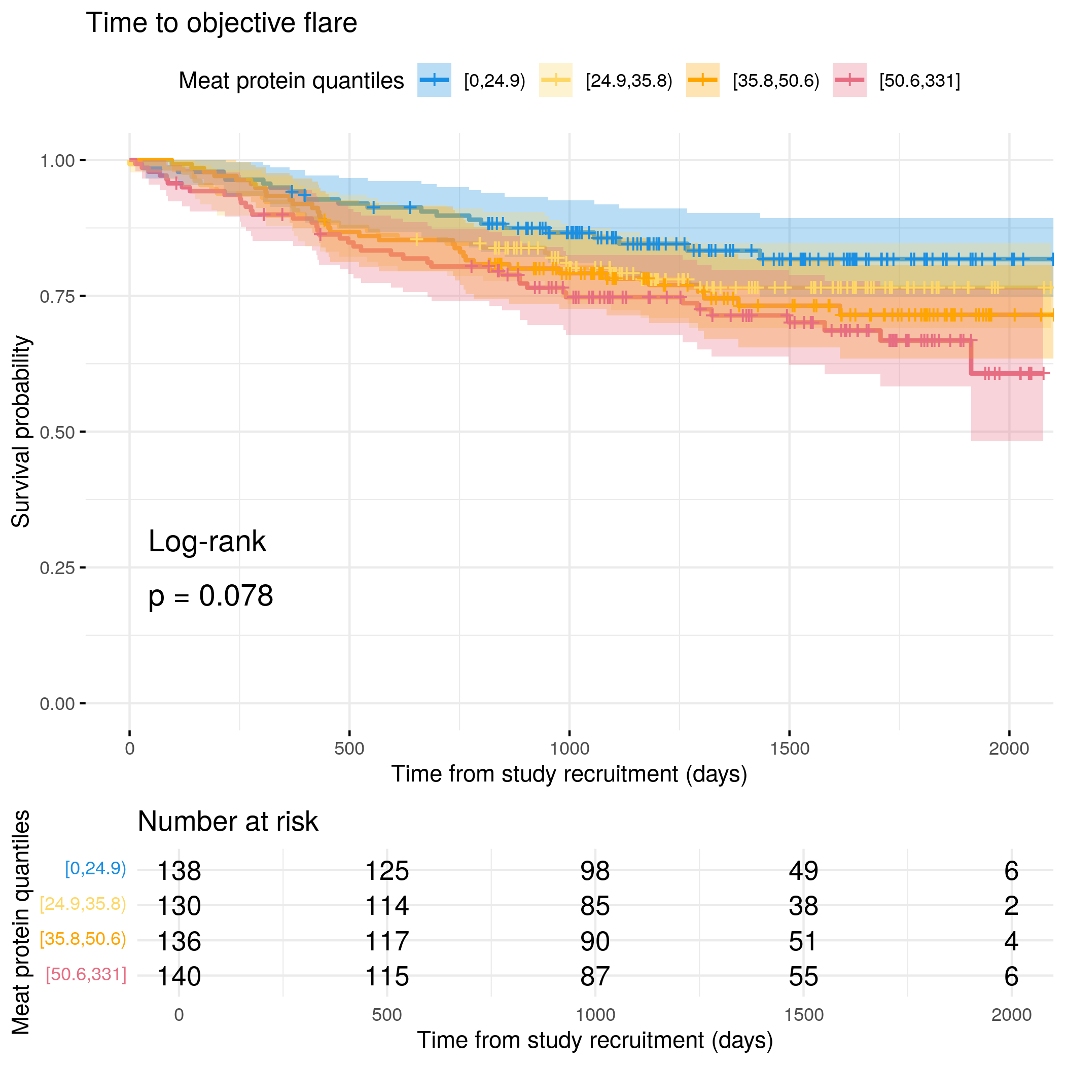
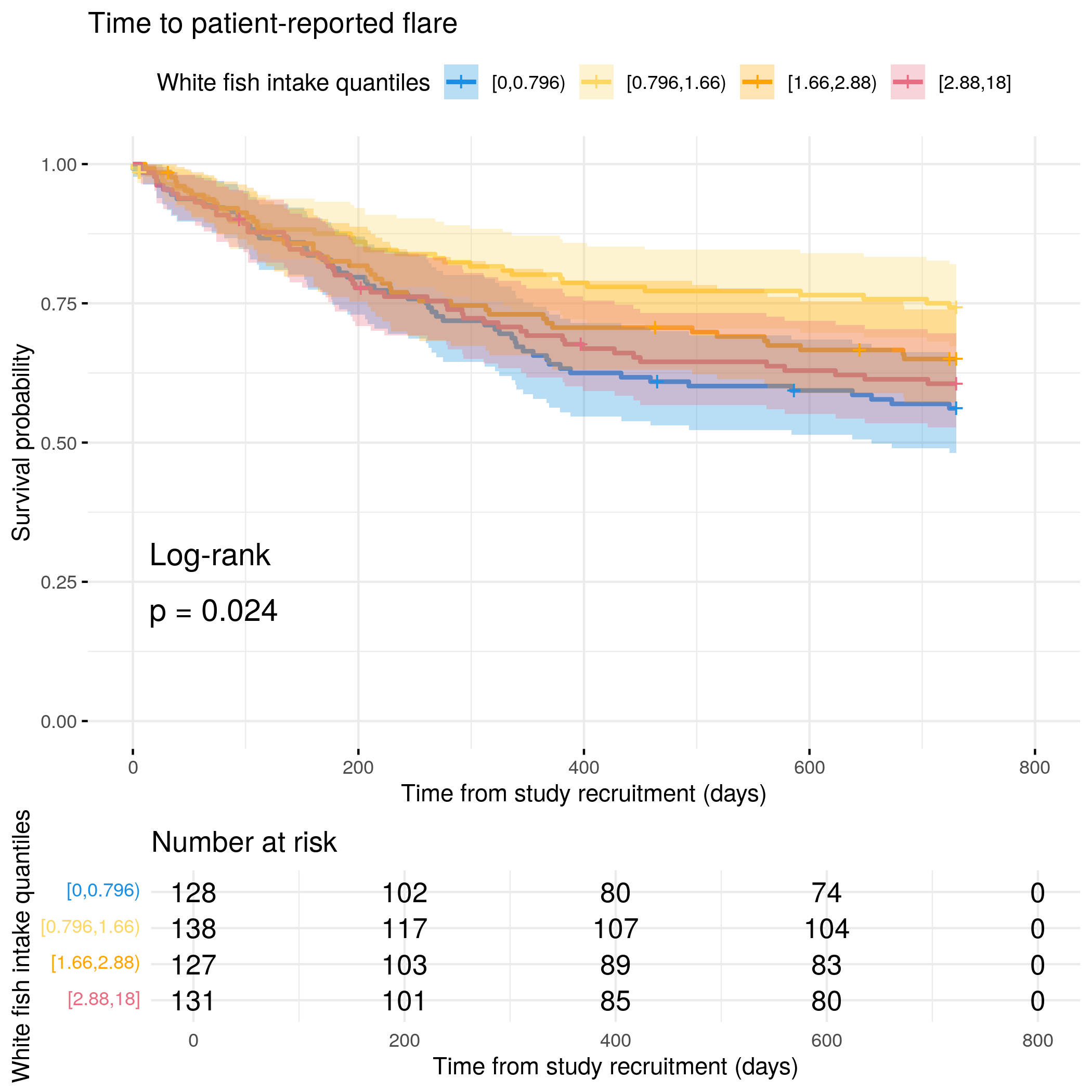
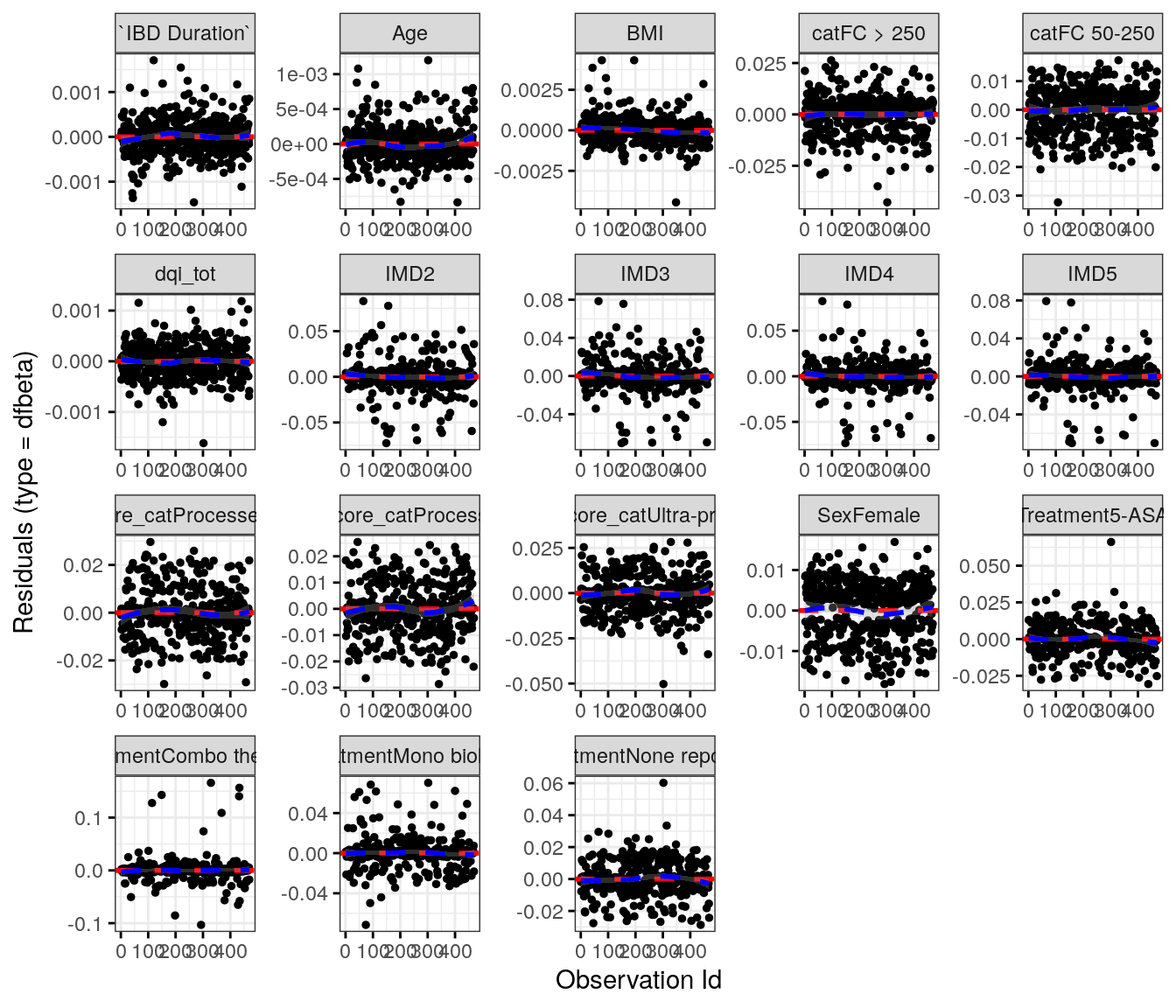
Protein intake from animal sources is not found to be significantly associated with flares in CD. However, there is evidence of an association for UC. At present, it is difficult to explore this in more detail (e.g. by meat type).
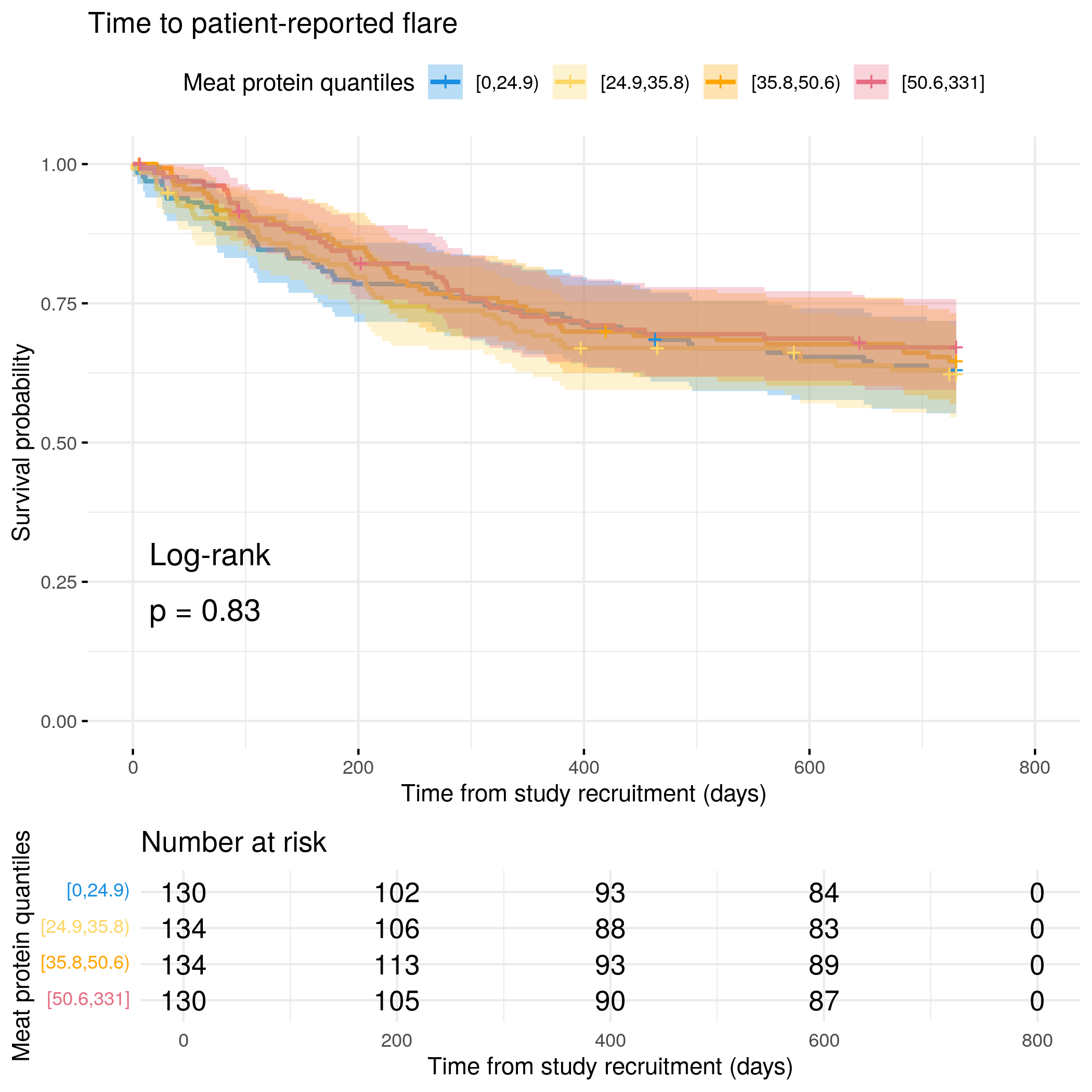
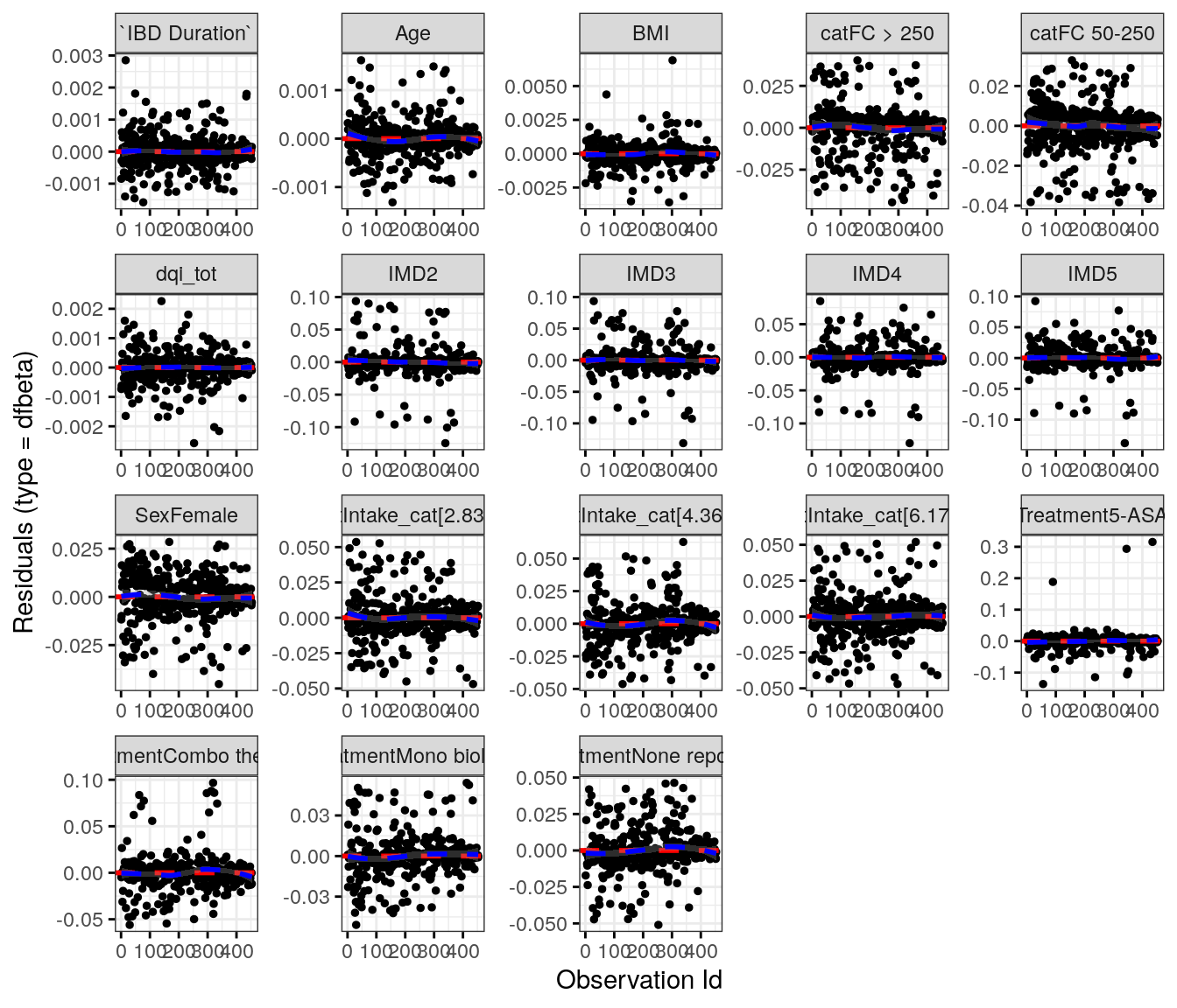
# Categorize meat protein by quantilesflare.cd.df<-categorize_by_quantiles(flare.cd.df, "Meat_sum", reference_data =flare.df)# Run survival analysis using utility functionanalysis_result<-run_survival_analysis( data =flare.cd.df, var_name ="Meat_sum", outcome_time ="softflare_time", outcome_event ="softflare", legend_title ="Meat protein quantiles", plot_base_path ="plots/cd/soft-flare/diet/meat", break_time_by =200)# Save plot as RDSsaveRDS(analysis_result$plot, paste0(paths$outdir, "meat-cd-soft.RDS"))# Run Cox model with categorical variablefit.me<-coxph(Surv(softflare_time, softflare)~Sex+cat+IMD+dqi_tot+Meat_sum_cat+frailty(SiteNo), control =coxph.control(outer.max =20), data =flare.cd.df)hrs<-broom::tidy(fit.me)|>filter(!grepl("^Sex|^cat|^IMD|^dqi_tot|^BMI|^frailty", term))|>mutate(diagnosis ="CD", flare ="Soft")|>relocate(diagnosis, flare)# Display plot and model summaryknitr::include_graphics("plots/cd/soft-flare/diet/meat.png")
Warning: `gather_()` was deprecated in tidyr 1.2.0.
ℹ Please use `gather()` instead.
ℹ The deprecated feature was likely used in the survminer package.
  Please report the issue at <https://github.com/kassambara/survminer/issues>.
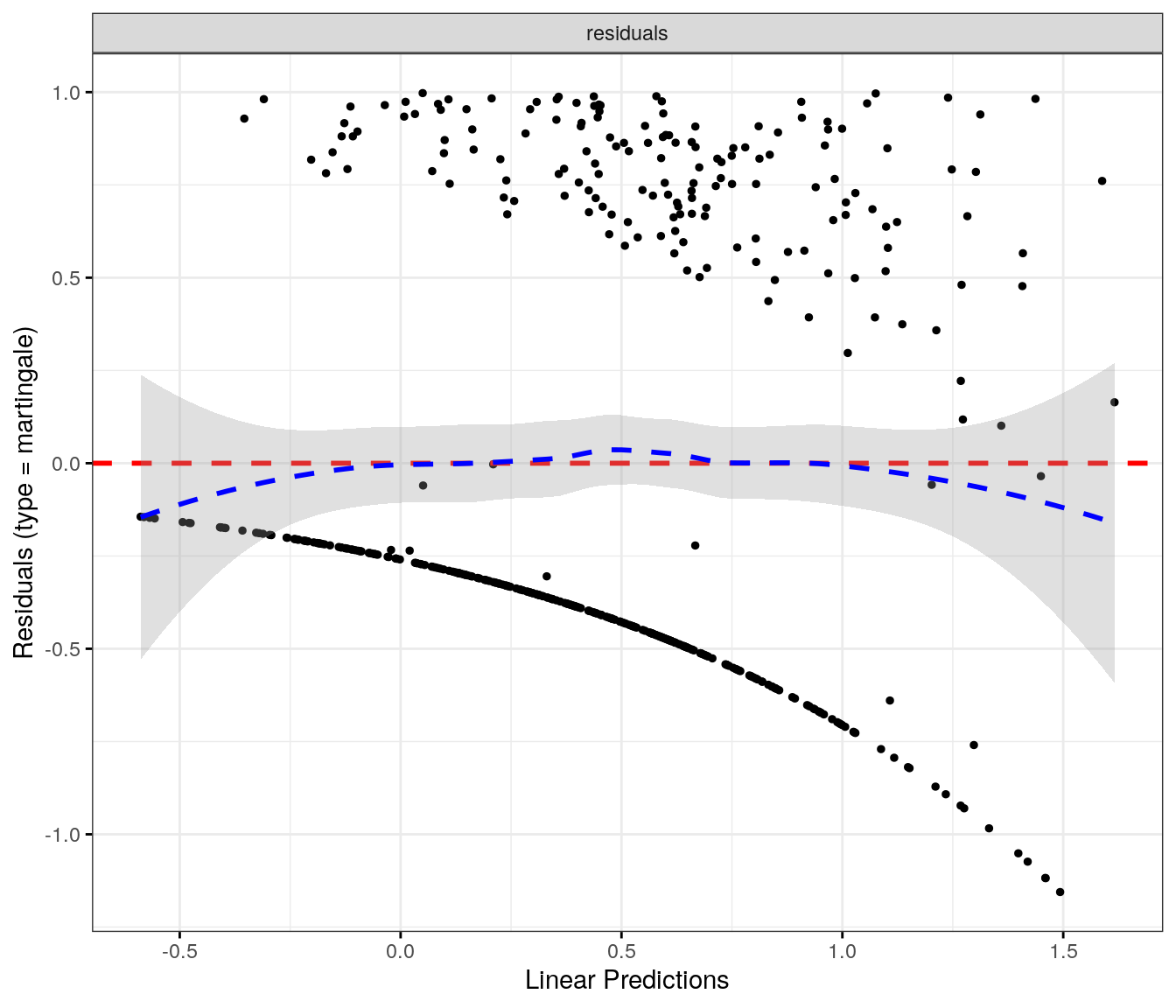
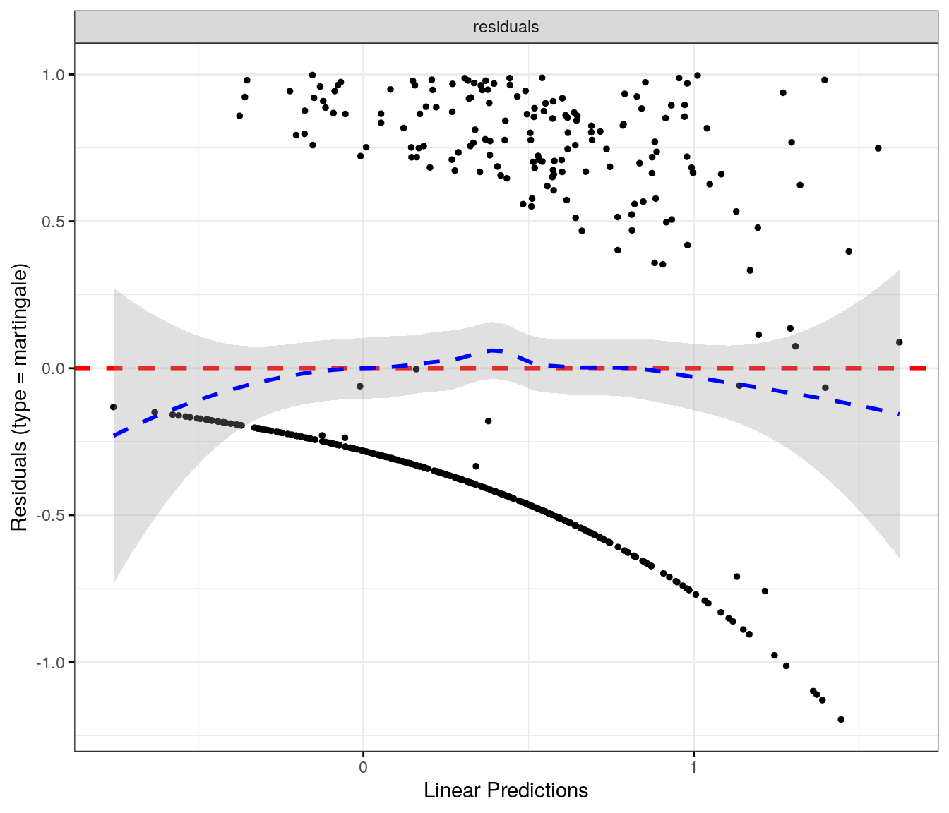
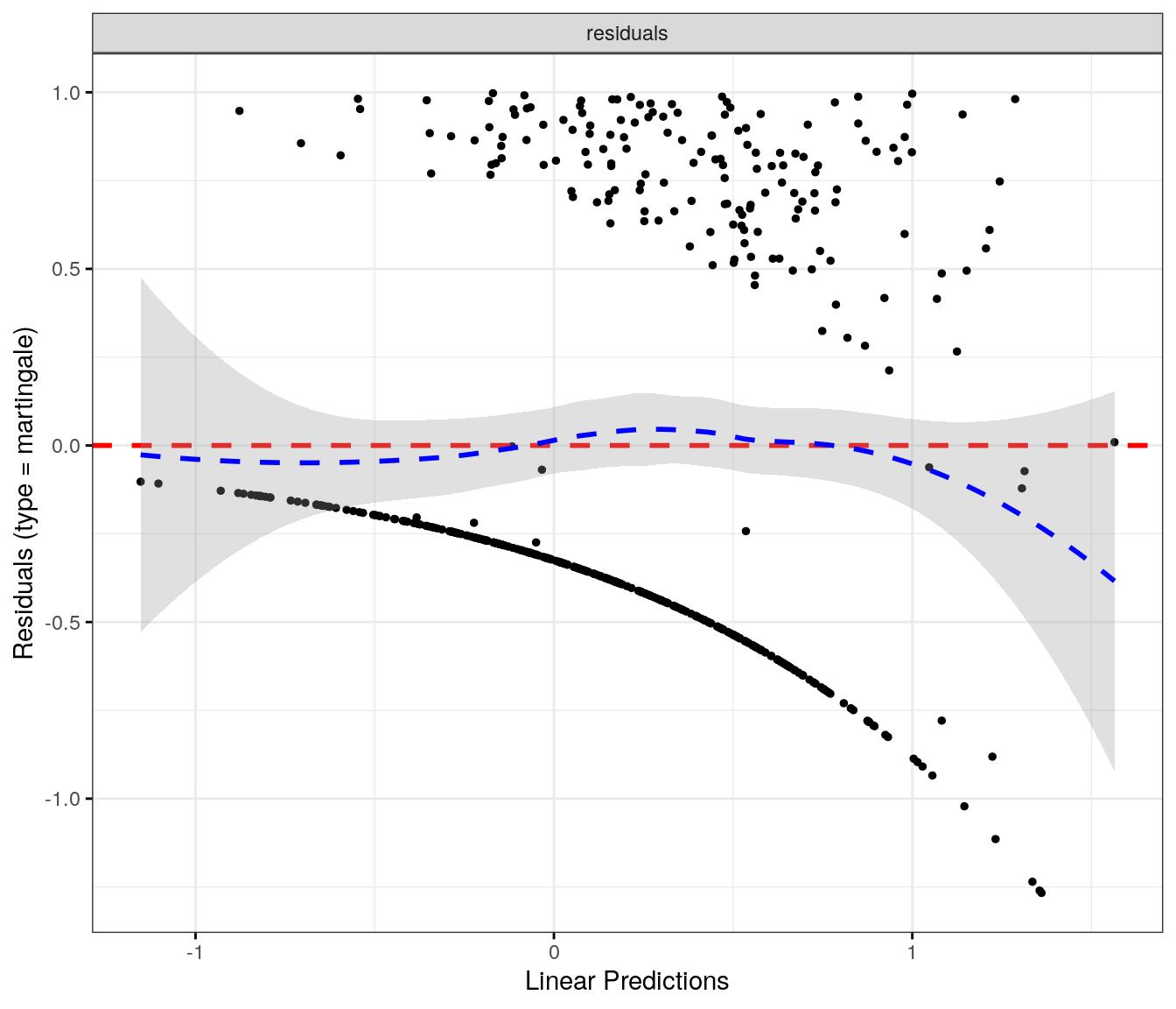
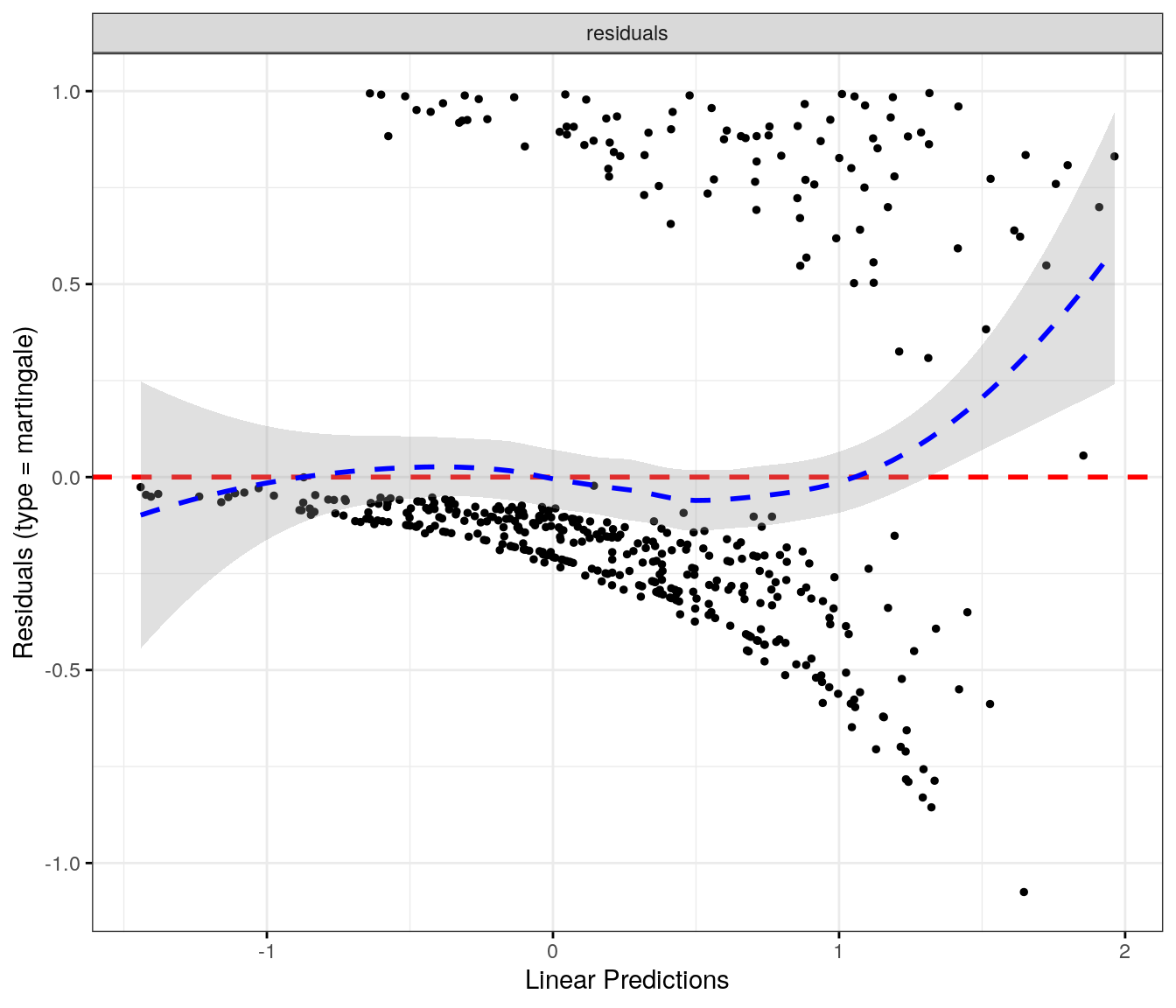
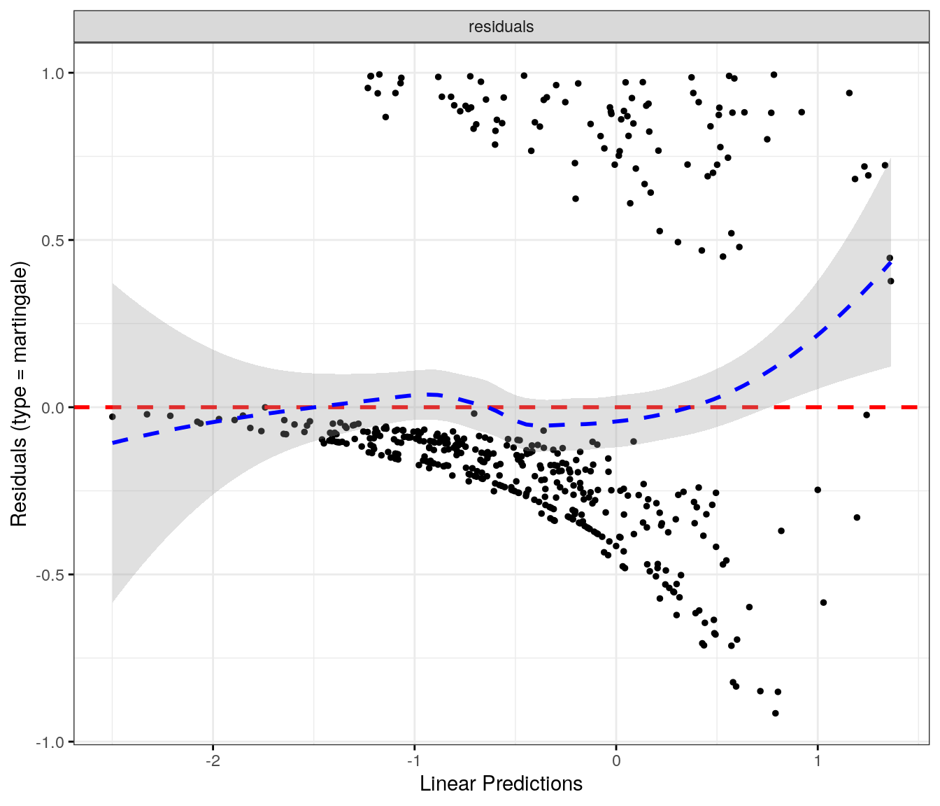
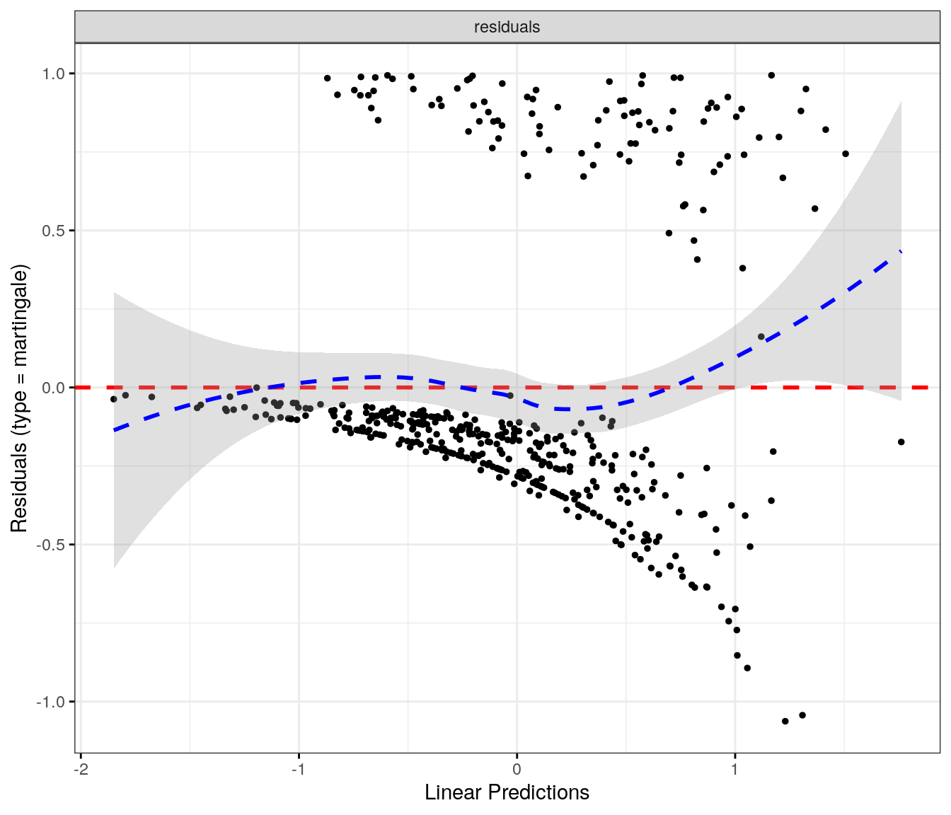
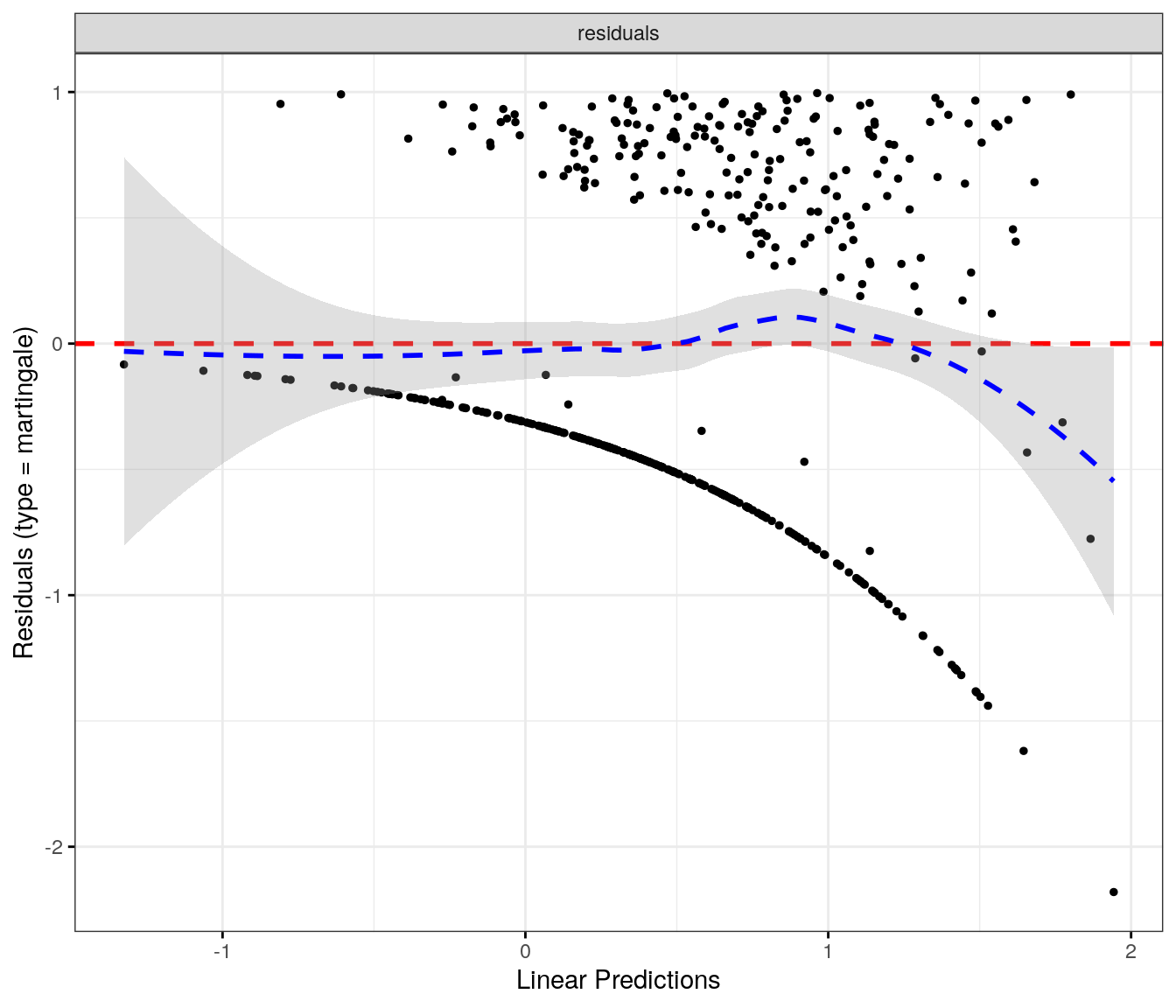
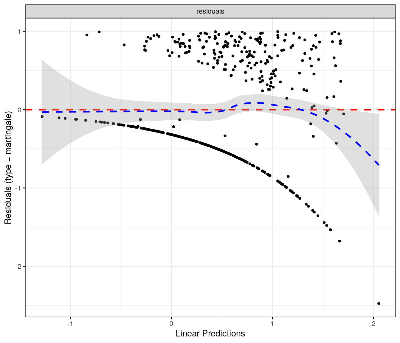
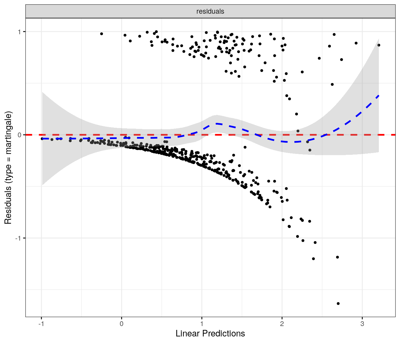
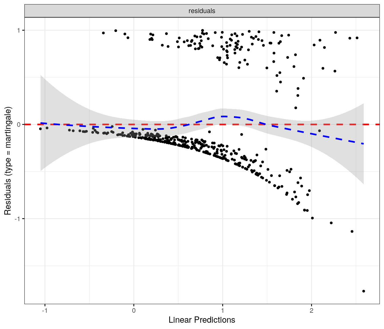
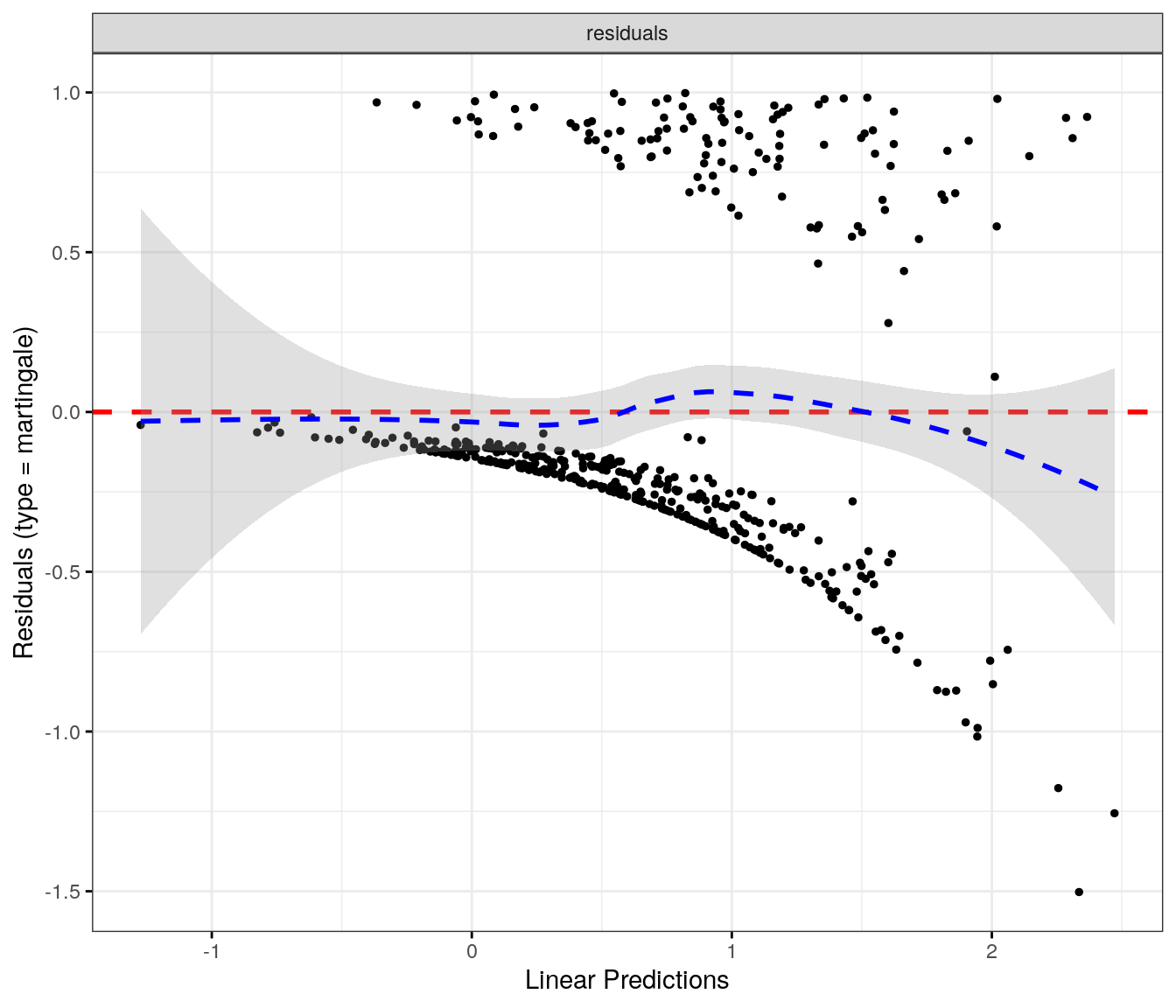
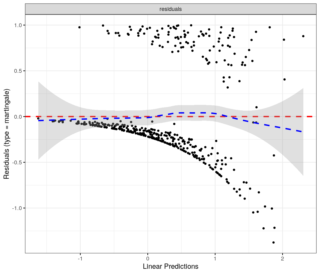
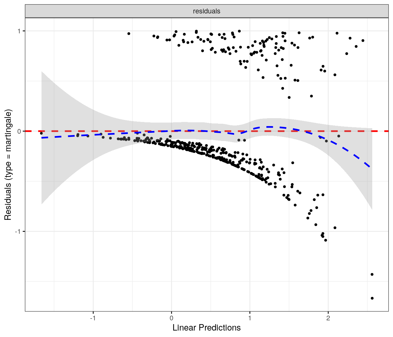
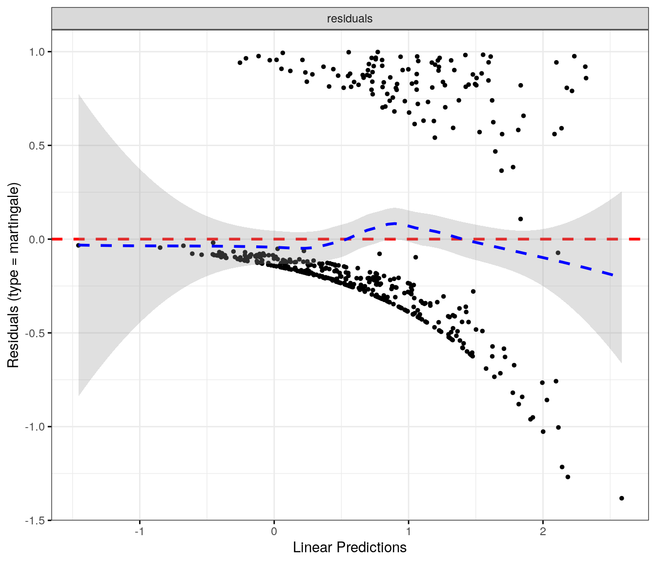
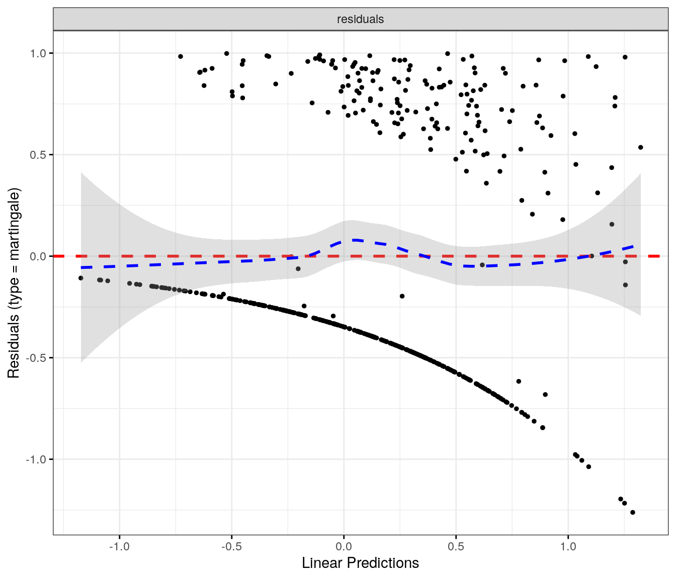
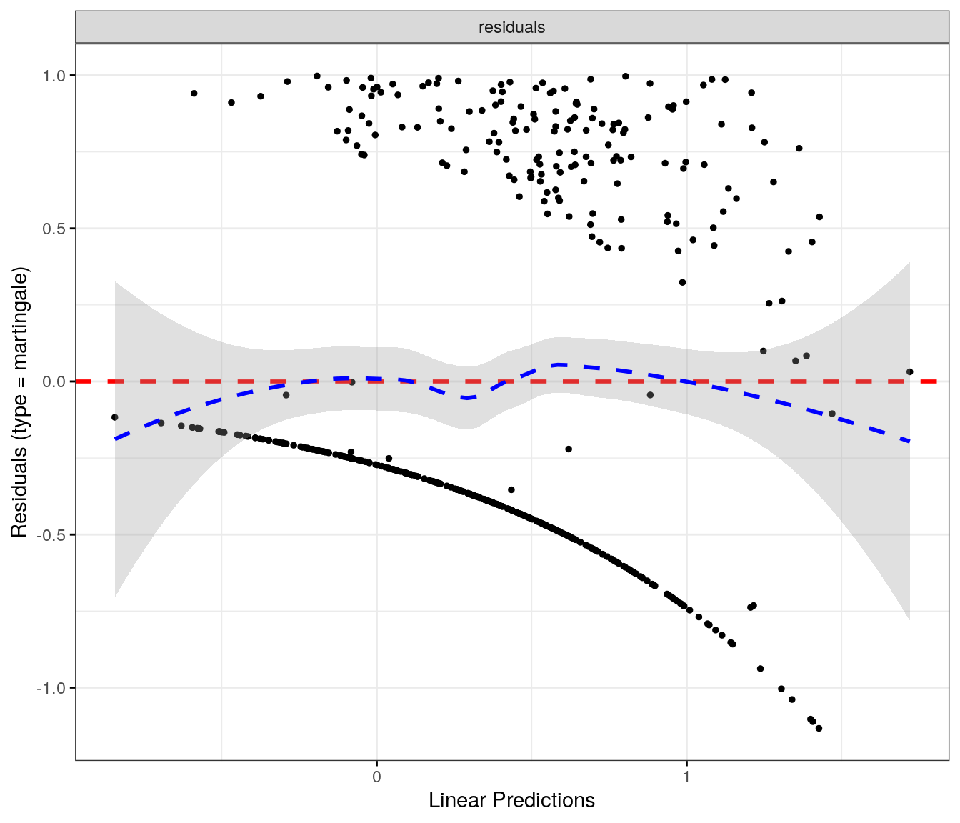
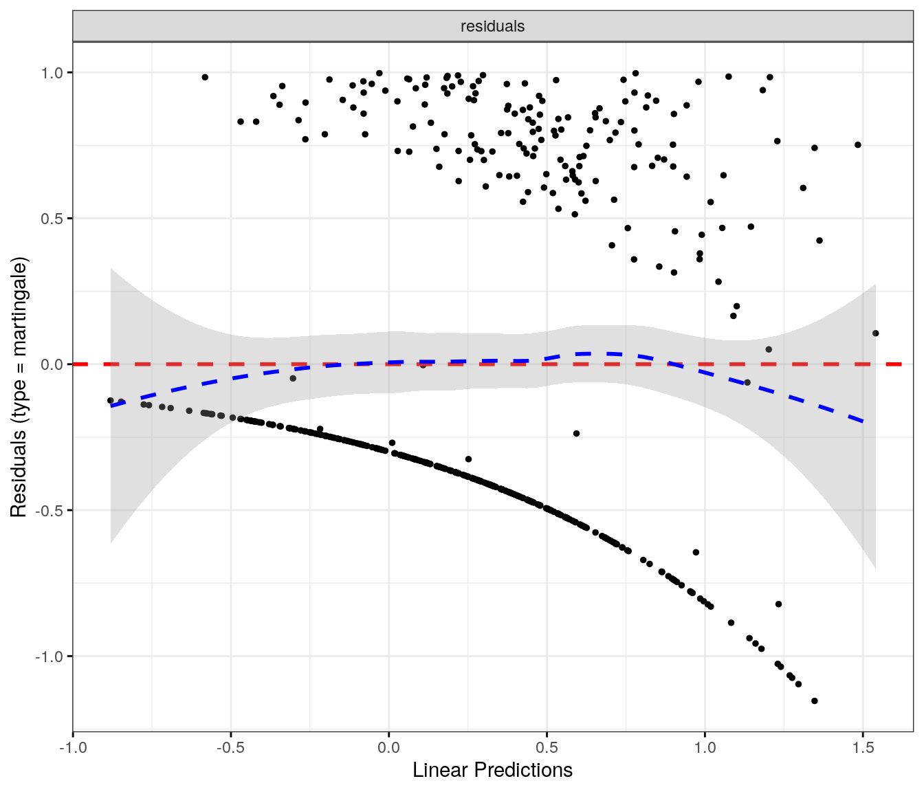
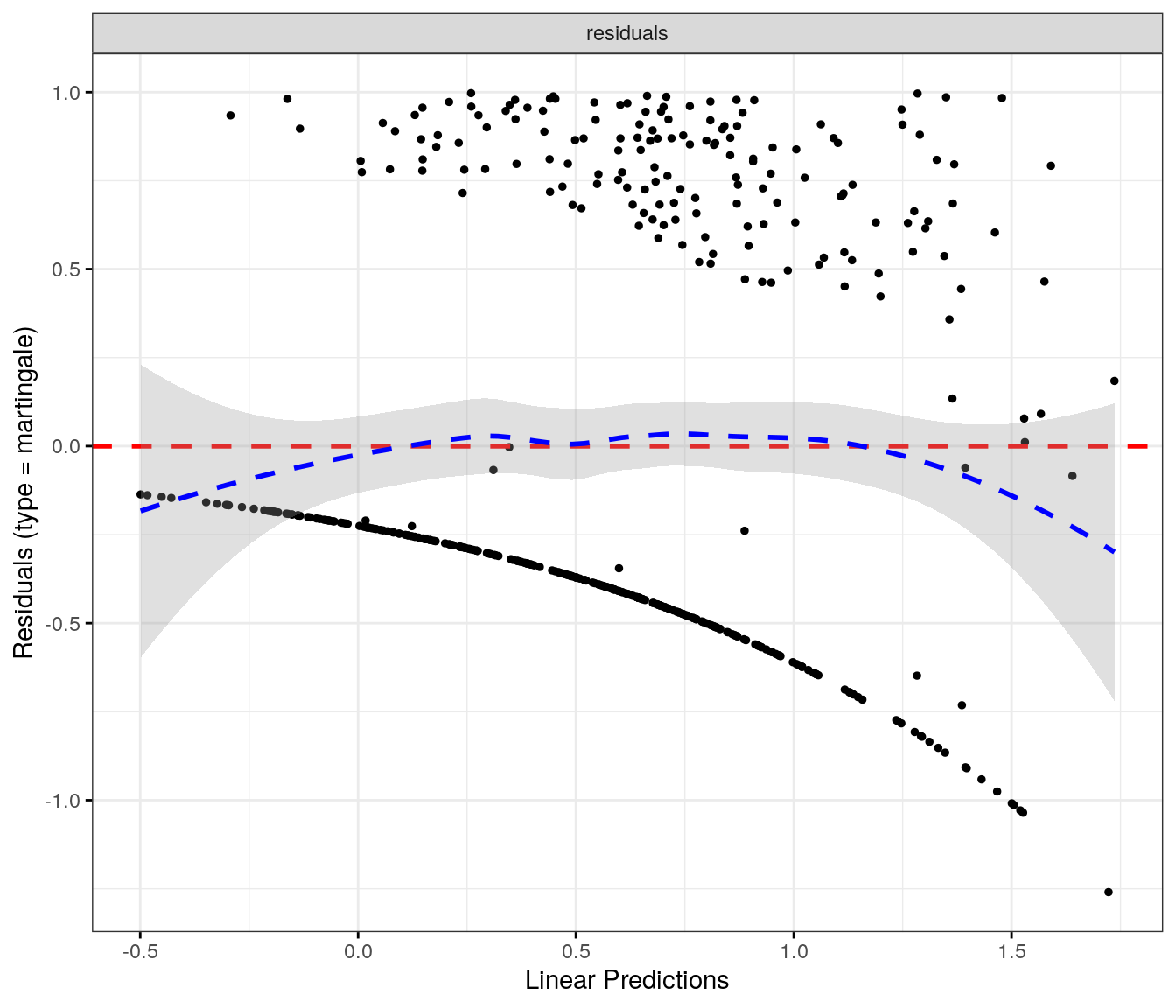
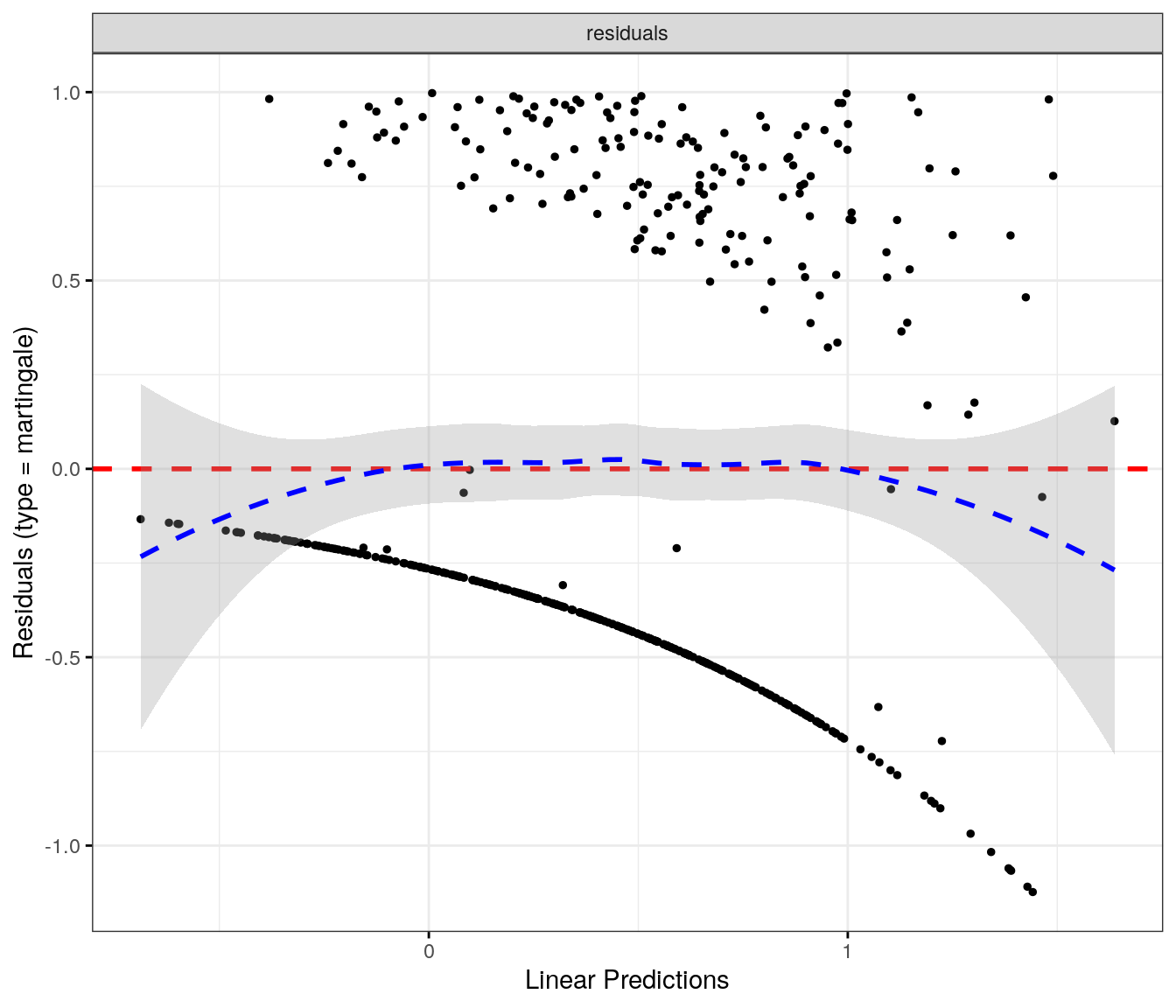
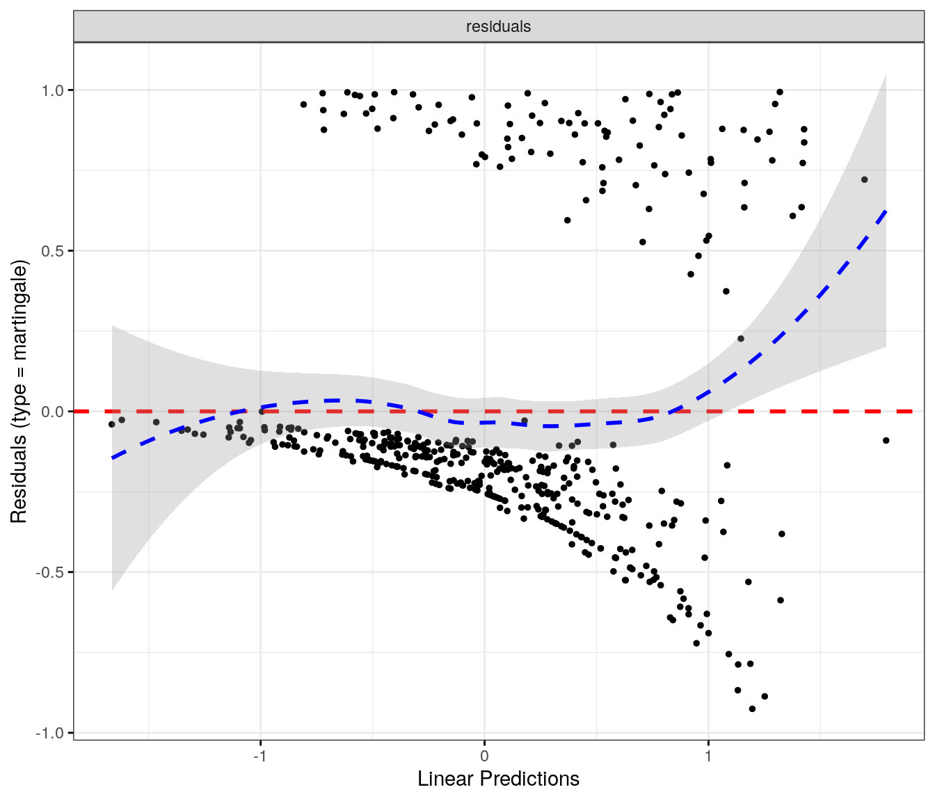
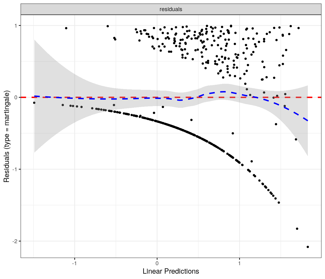
`geom_smooth()` using formula = 'y ~ x'
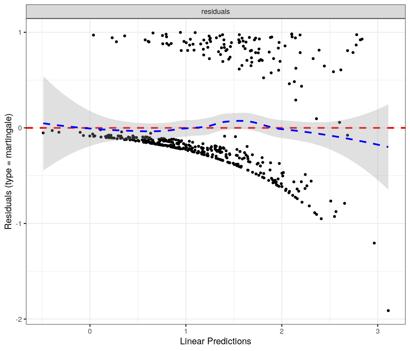
`geom_smooth()` using formula = 'y ~ x'
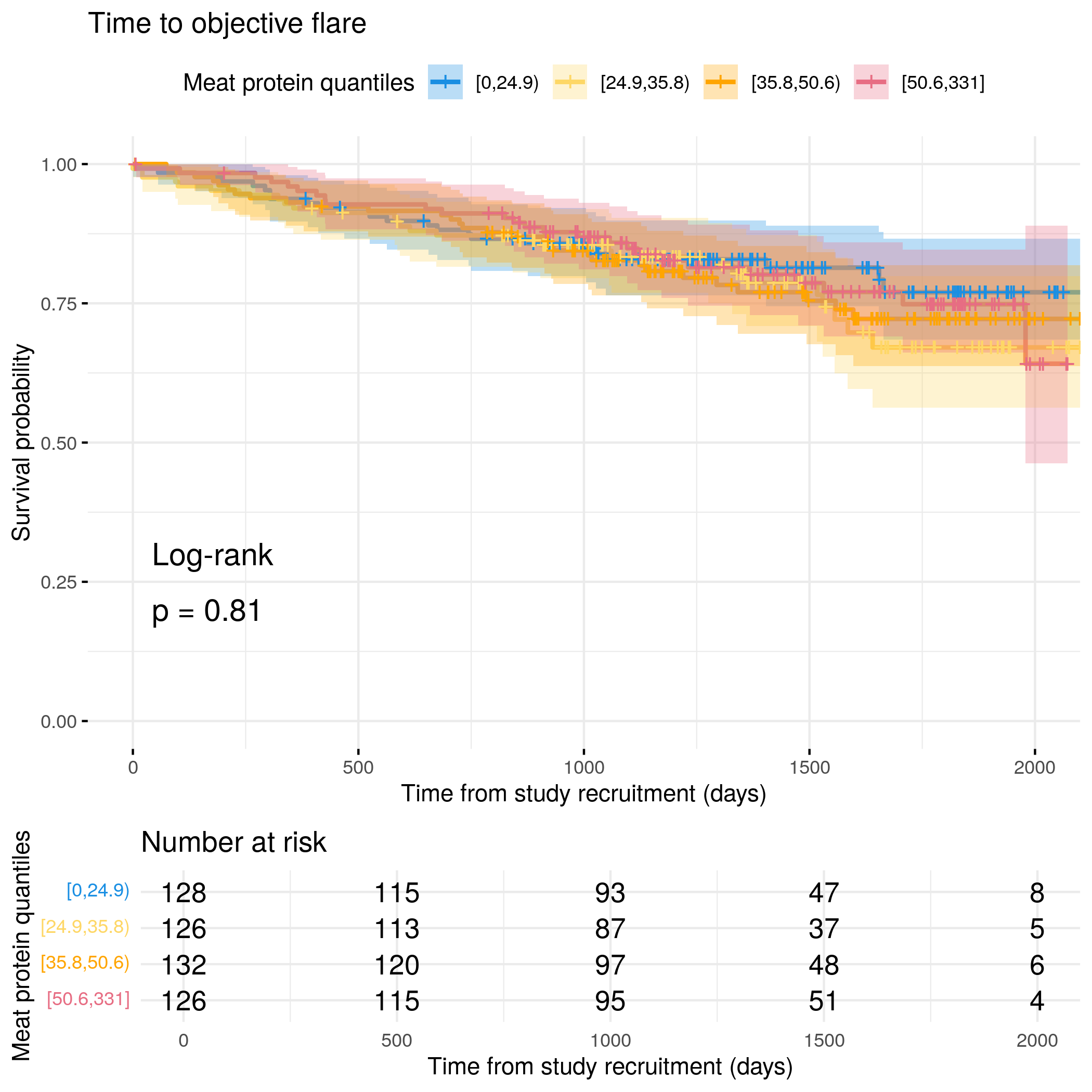
# Run survival analysis using utility function for objective flareanalysis_result<-run_survival_analysis( data =flare.cd.df, var_name ="Meat_sum", outcome_time ="hardflare_time", outcome_event ="hardflare", legend_title ="Meat protein quantiles", plot_base_path ="plots/cd/hard-flare/diet/meat", break_time_by =500)# Save plot as RDSsaveRDS(analysis_result$plot, paste0(paths$outdir, "meat-cd-hard.RDS"))# Run Cox model with categorical variablefit.me<-coxph(Surv(hardflare_time, hardflare)~Sex+cat+IMD+dqi_tot+Meat_sum_cat+frailty(SiteNo), control =coxph.control(outer.max =20), data =flare.cd.df)hrs<-rbind(hrs, broom::tidy(fit.me)|>filter(!grepl("^Sex|^cat|^IMD|^dqi_tot|^BMI|^frailty", term))|>mutate(diagnosis ="CD", flare ="Hard")|>relocate(diagnosis, flare))# Display plot and model summaryknitr::include_graphics("plots/cd/hard-flare/diet/meat.png")
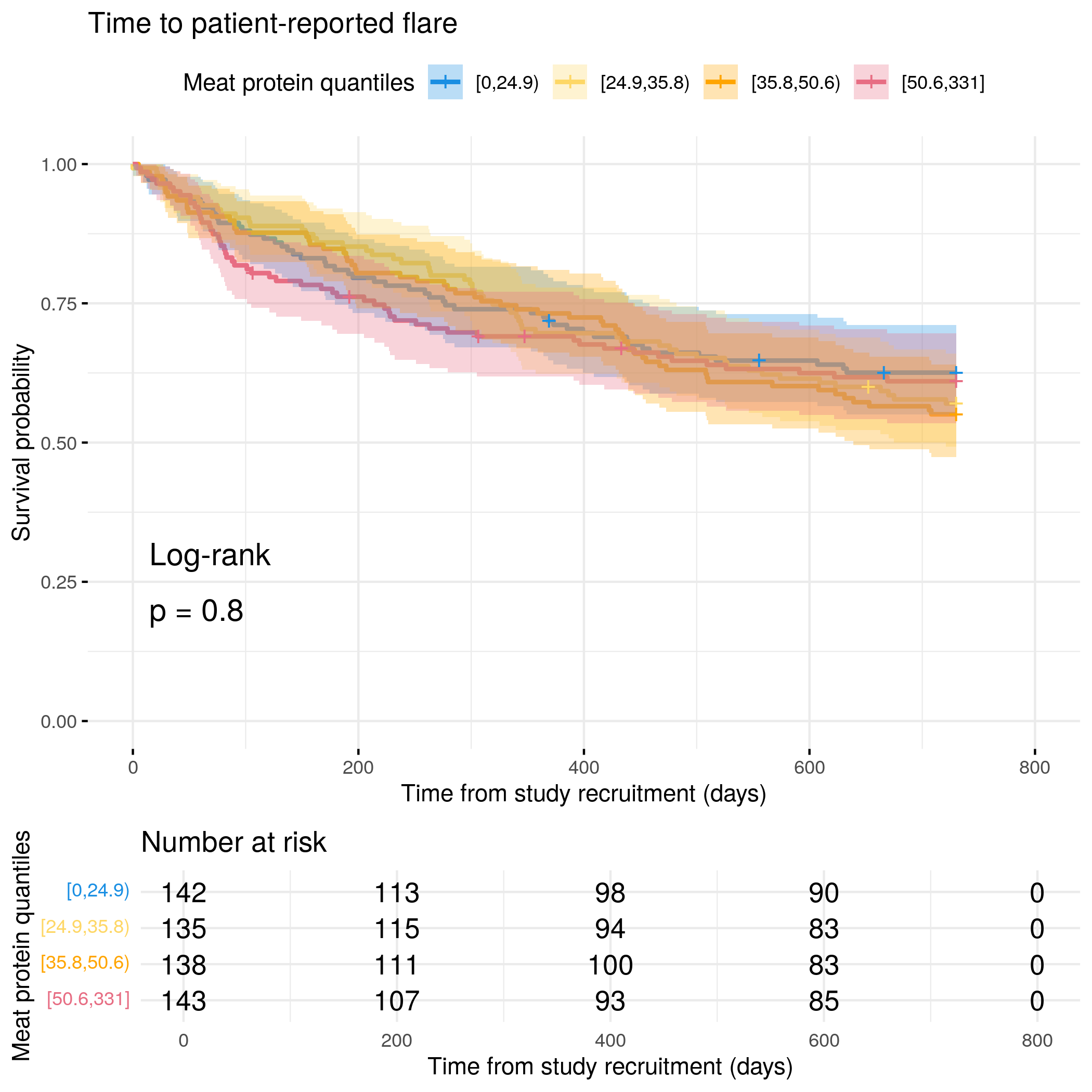
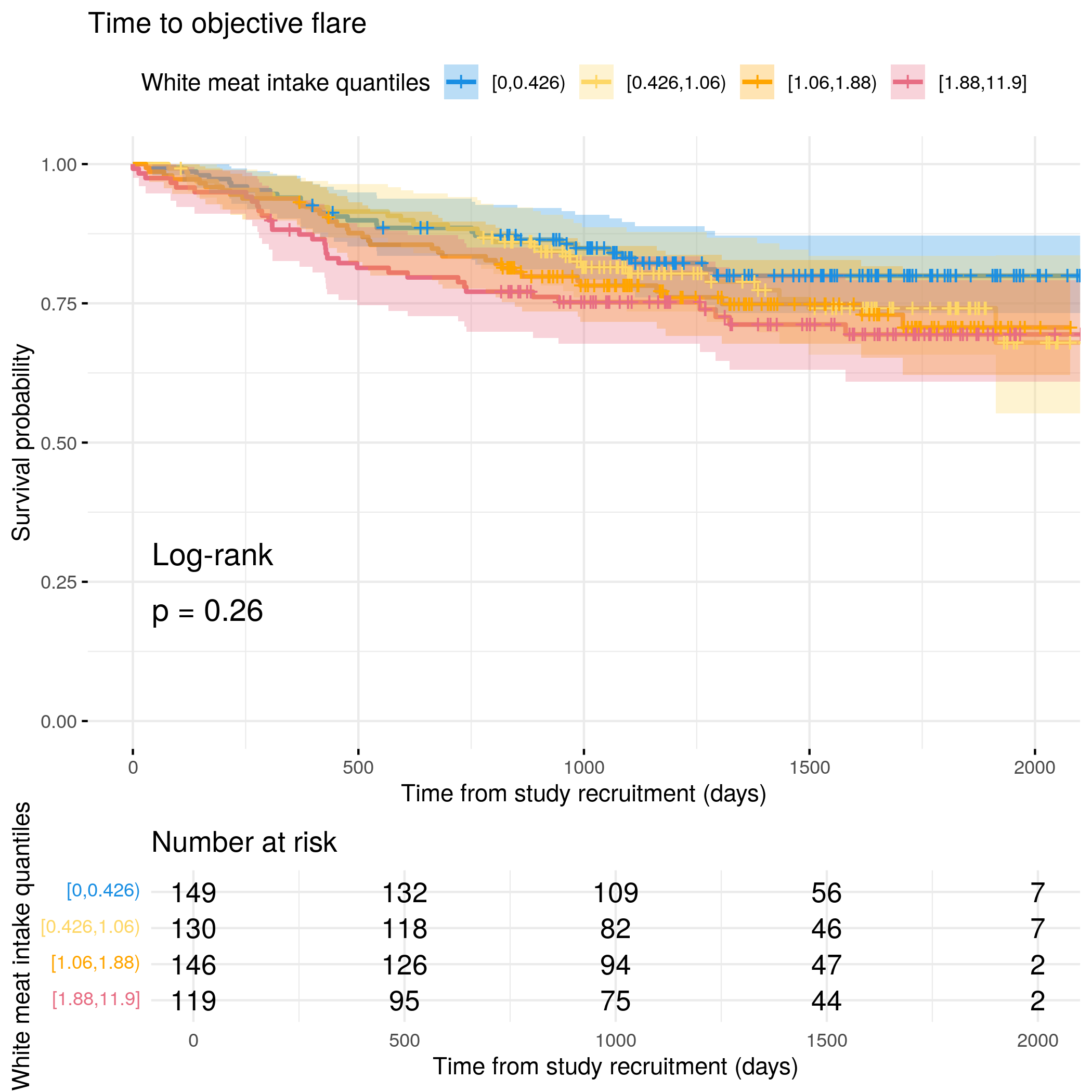
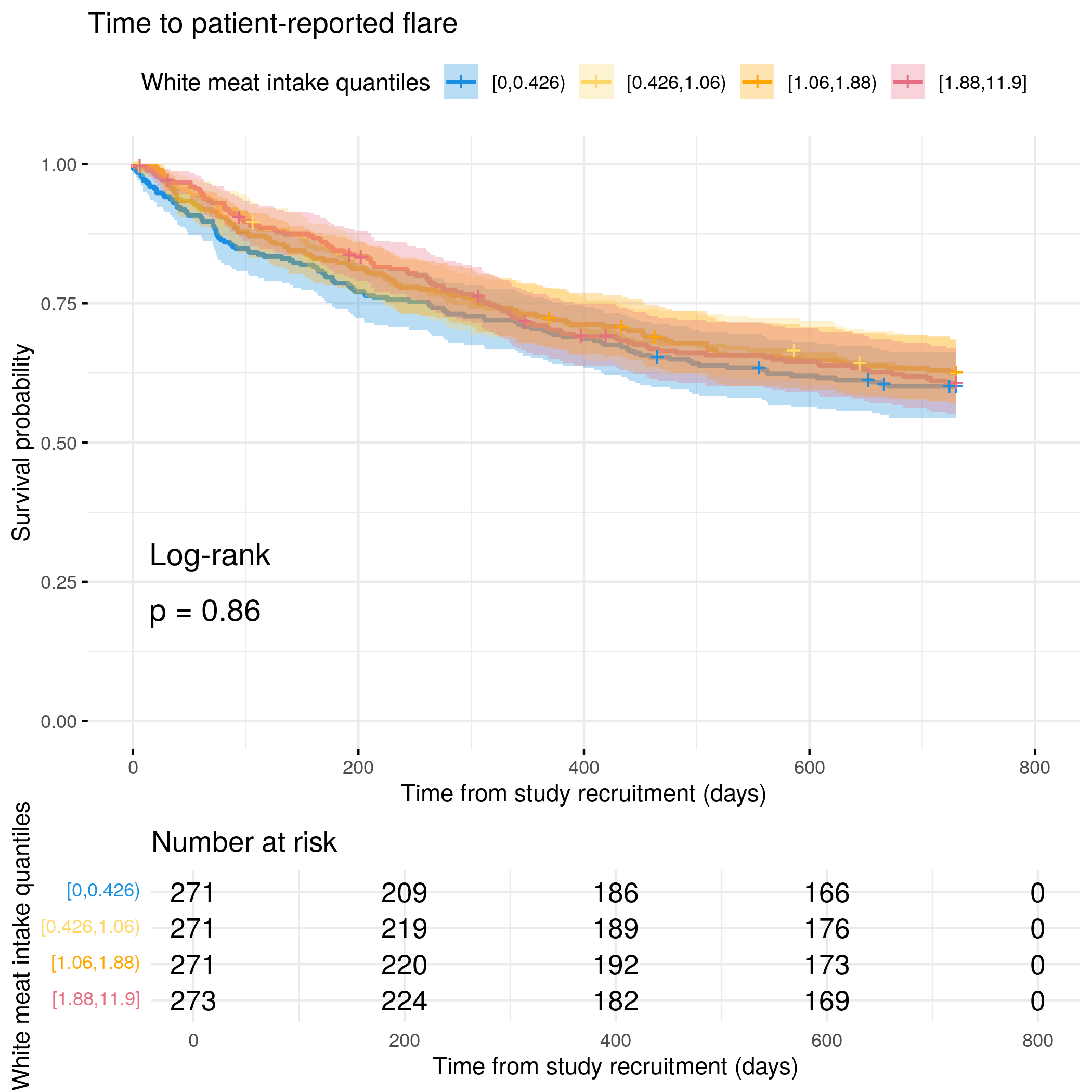
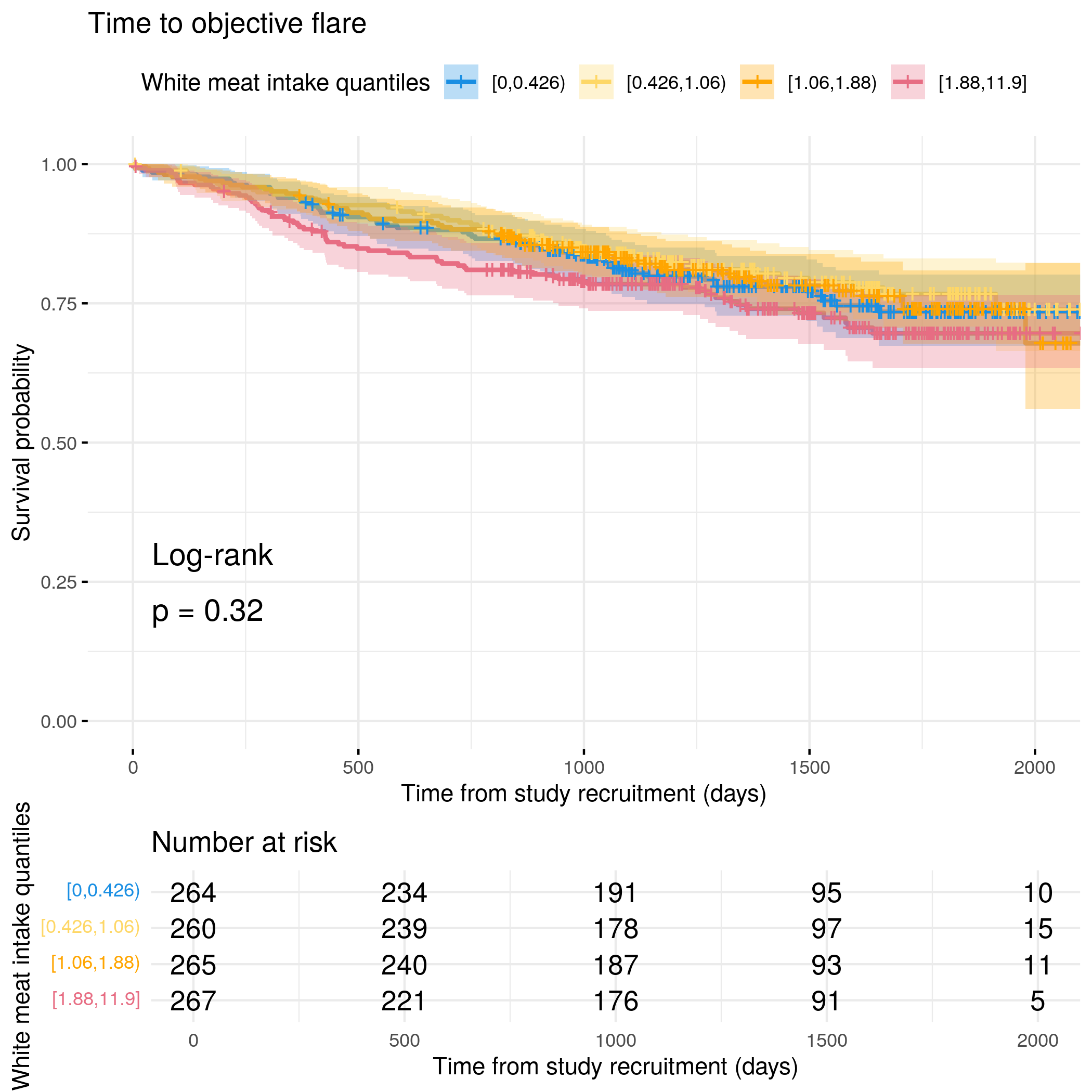
# Categorize meat protein by quantilesflare.uc.df<-categorize_by_quantiles(flare.uc.df, "Meat_sum", reference_data =flare.df)# Run survival analysis using utility functionanalysis_result<-run_survival_analysis( data =flare.uc.df, var_name ="Meat_sum", outcome_time ="softflare_time", outcome_event ="softflare", legend_title ="Meat protein quantiles", plot_base_path ="plots/uc/soft-flare/diet/meat", break_time_by =200)# Save plot as RDSsaveRDS(analysis_result$plot, paste0(paths$outdir, "meat-uc-soft.RDS"))# Run Cox model with categorical variablefit.me<-coxph(Surv(softflare_time, softflare)~Sex+cat+IMD+dqi_tot+Meat_sum_cat+frailty(SiteNo), control =coxph.control(outer.max =20), data =flare.uc.df)hrs<-rbind(hrs, broom::tidy(fit.me)|>filter(!grepl("^Sex|^cat|^IMD|^dqi_tot|^BMI|^frailty", term))|>mutate(diagnosis ="UC", flare ="Soft")|>relocate(diagnosis, flare))# Display plot and model summaryknitr::include_graphics("plots/uc/soft-flare/diet/meat.png")
# Run survival analysis using utility function for objective flareanalysis_result<-run_survival_analysis( data =flare.uc.df, var_name ="Meat_sum", outcome_time ="hardflare_time", outcome_event ="hardflare", legend_title ="Meat protein quantiles", plot_base_path ="plots/uc/hard-flare/diet/meat", break_time_by =500)# Save plot as RDSsaveRDS(analysis_result$plot, paste0(paths$outdir, "meat-uc-hard.RDS"))# Run Cox model with categorical variablefit.me<-coxph(Surv(hardflare_time, hardflare)~Sex+cat+IMD+dqi_tot+Meat_sum_cat+frailty(SiteNo), control =coxph.control(outer.max =20), data =flare.uc.df)hrs<-rbind(hrs, broom::tidy(fit.me)|>filter(!grepl("^Sex|^cat|^IMD|^dqi_tot|^BMI|^frailty", term))|>mutate(diagnosis ="UC", flare ="Hard")|>relocate(diagnosis, flare))# Display plot and model summaryknitr::include_graphics("plots/uc/hard-flare/diet/meat.png")
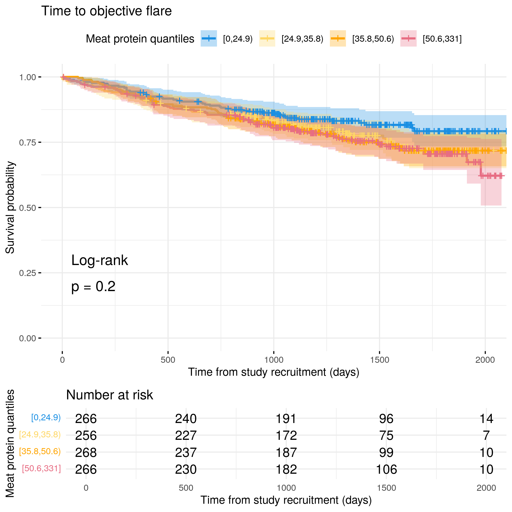
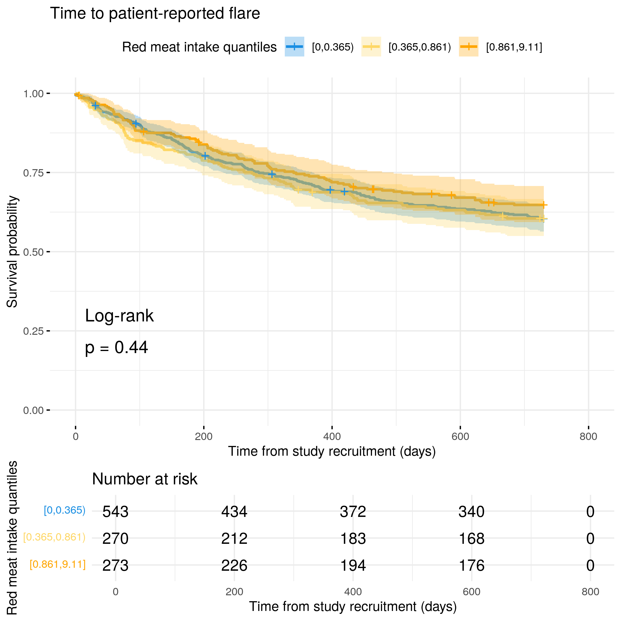
# Categorize meat protein by quantilesflare.df<-categorize_by_quantiles(flare.df, "Meat_sum", reference_data =flare.df)# Run survival analysis using utility functionanalysis_result<-run_survival_analysis( data =flare.df, var_name ="Meat_sum", outcome_time ="softflare_time", outcome_event ="softflare", legend_title ="Meat protein quantiles", plot_base_path ="plots/ibd/soft-flare/diet/meat", break_time_by =200)# Run Cox model with categorical variablefit.me<-coxph(Surv(softflare_time, softflare)~Sex+cat+IMD+dqi_tot+Meat_sum_cat+frailty(SiteNo), control =coxph.control(outer.max =20), data =flare.df)hrs<-rbind(hrs, broom::tidy(fit.me)|>filter(!grepl("^Sex|^cat|^IMD|^dqi_tot|^BMI|^frailty", term))|>mutate(diagnosis ="IBD", flare ="Soft")|>relocate(diagnosis, flare))# Display plot and model summaryknitr::include_graphics("plots/ibd/soft-flare/diet/meat.png")
# Run survival analysis using utility function for objective flareanalysis_result<-run_survival_analysis( data =flare.df, var_name ="Meat_sum", outcome_time ="hardflare_time", outcome_event ="hardflare", legend_title ="Meat protein quantiles", plot_base_path ="plots/ibd/hard-flare/diet/meat", break_time_by =500)# Run Cox model with categorical variablefit.me<-coxph(Surv(hardflare_time, hardflare)~Sex+cat+IMD+dqi_tot+Meat_sum_cat+frailty(SiteNo), control =coxph.control(outer.max =20), data =flare.df)hrs<-rbind(hrs, broom::tidy(fit.me)|>filter(!grepl("^Sex|^cat|^IMD|^dqi_tot|^BMI|^frailty", term))|>mutate(diagnosis ="IBD", flare ="Hard")|>relocate(diagnosis, flare))# Display plot and model summaryknitr::include_graphics("plots/ibd/hard-flare/diet/meat.png")
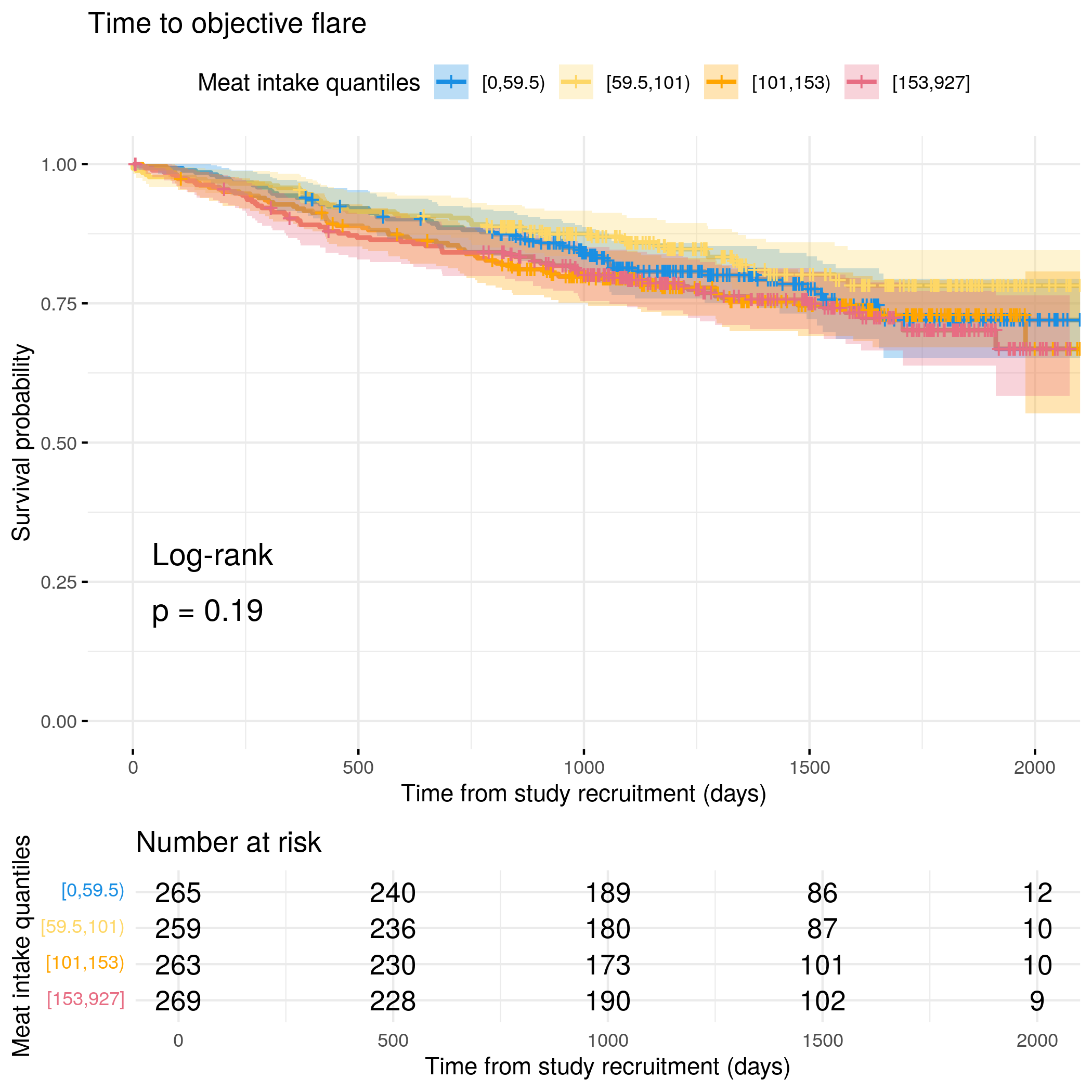
# Categorize overall meat intake by quantilesflare.cd.df<-categorize_by_quantiles(flare.cd.df, "meat_overall", reference_data =flare.df)# Run survival analysis using utility functionanalysis_result<-run_survival_analysis( data =flare.cd.df, var_name ="meat_overall", outcome_time ="softflare_time", outcome_event ="softflare", legend_title ="Meat intake quantiles", plot_base_path ="plots/cd/soft-flare/diet/meat_overall", break_time_by =200)# Save plot as RDSsaveRDS(analysis_result$plot, paste0(paths$outdir, "meat-overall-cd-soft.RDS"))# Run Cox model with categorical variablefit.me<-coxph(Surv(softflare_time, softflare)~Sex+cat+IMD+dqi_tot+meat_overall_cat+frailty(SiteNo), control =coxph.control(outer.max =20), data =flare.cd.df)hrs<-rbind(hrs, broom::tidy(fit.me)|>filter(!grepl("^Sex|^cat|^IMD|^dqi_tot|^BMI|^frailty", term))|>mutate(diagnosis ="CD", flare ="Soft")|>relocate(diagnosis, flare))# Display plot and model summaryknitr::include_graphics("plots/cd/soft-flare/diet/meat_overall.png")
# Run survival analysis using utility function for objective flareanalysis_result<-run_survival_analysis( data =flare.cd.df, var_name ="meat_overall", outcome_time ="hardflare_time", outcome_event ="hardflare", legend_title ="Meat intake quantiles", plot_base_path ="plots/cd/hard-flare/diet/meat_overall", break_time_by =500)# Save plot as RDSsaveRDS(analysis_result$plot, paste0(paths$outdir, "meat-overall-cd-hard.RDS"))# Run Cox model with categorical variablefit.me<-coxph(Surv(hardflare_time, hardflare)~Sex+cat+IMD+dqi_tot+meat_overall_cat+frailty(SiteNo), control =coxph.control(outer.max =20), data =flare.cd.df)hrs<-rbind(hrs, broom::tidy(fit.me)|>filter(!grepl("^Sex|^cat|^IMD|^dqi_tot|^BMI|^frailty", term))|>mutate(diagnosis ="CD", flare ="Hard")|>relocate(diagnosis, flare))# Display plot and model summaryknitr::include_graphics("plots/cd/hard-flare/diet/meat_overall.png")
# Categorize overall meat intake by quantilesflare.uc.df<-categorize_by_quantiles(flare.uc.df, "meat_overall", reference_data =flare.df)# Run survival analysis using utility functionanalysis_result<-run_survival_analysis( data =flare.uc.df, var_name ="meat_overall", outcome_time ="softflare_time", outcome_event ="softflare", legend_title ="Meat intake quantiles", plot_base_path ="plots/uc/soft-flare/diet/meat_overall", break_time_by =200)# Save plot as RDSsaveRDS(analysis_result$plot, paste0(paths$outdir, "meat-overall-uc-soft.RDS"))# Run Cox model with categorical variablefit.me<-coxph(Surv(softflare_time, softflare)~Sex+cat+IMD+dqi_tot+meat_overall_cat+frailty(SiteNo), control =coxph.control(outer.max =20), data =flare.uc.df)hrs<-rbind(hrs, broom::tidy(fit.me)|>filter(!grepl("^Sex|^cat|^IMD|^dqi_tot|^BMI|^frailty", term))|>mutate(diagnosis ="UC", flare ="Soft")|>relocate(diagnosis, flare))# Display plot and model summaryknitr::include_graphics("plots/uc/soft-flare/diet/meat_overall.png")
# Run survival analysis using utility function for objective flareanalysis_result<-run_survival_analysis( data =flare.uc.df, var_name ="meat_overall", outcome_time ="hardflare_time", outcome_event ="hardflare", legend_title ="Meat intake quantiles", plot_base_path ="plots/uc/hard-flare/diet/meat_overall", break_time_by =500)# Save plot as RDSsaveRDS(analysis_result$plot, paste0(paths$outdir, "meat-overall-uc-hard.RDS"))# Run Cox model with categorical variablefit.me<-coxph(Surv(hardflare_time, hardflare)~Sex+cat+IMD+dqi_tot+meat_overall_cat+frailty(SiteNo), control =coxph.control(outer.max =20), data =flare.uc.df)hrs<-rbind(hrs, broom::tidy(fit.me)|>filter(!grepl("^Sex|^cat|^IMD|^dqi_tot|^BMI|^frailty", term))|>mutate(diagnosis ="UC", flare ="Hard")|>relocate(diagnosis, flare))# Display plot and model summaryknitr::include_graphics("plots/uc/hard-flare/diet/meat_overall.png")
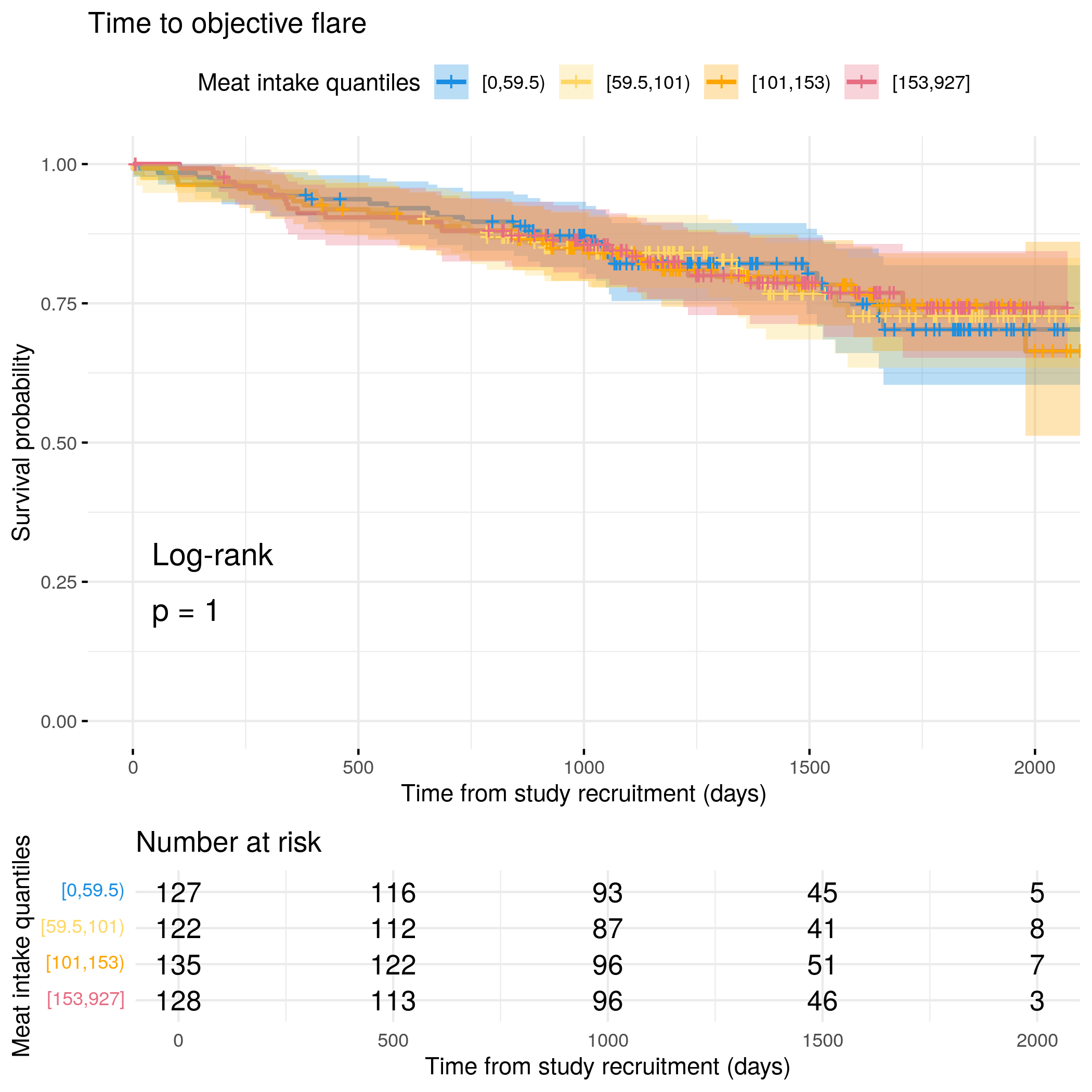
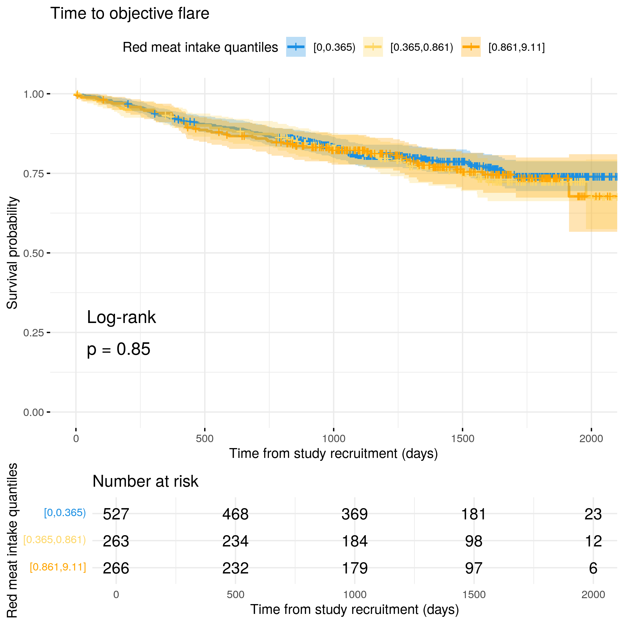
# Categorize overall meat intake by quantilesflare.df<-categorize_by_quantiles(flare.df, "meat_overall", reference_data =flare.df)# Run survival analysis using utility functionanalysis_result<-run_survival_analysis( data =flare.df, var_name ="meat_overall", outcome_time ="softflare_time", outcome_event ="softflare", legend_title ="Meat intake quantiles", plot_base_path ="plots/ibd/soft-flare/diet/meat_overall", break_time_by =200)# Run Cox model with categorical variablefit.me<-coxph(Surv(softflare_time, softflare)~Sex+cat+IMD+dqi_tot+meat_overall_cat+frailty(SiteNo), control =coxph.control(outer.max =20), data =flare.df)hrs<-rbind(hrs, broom::tidy(fit.me)|>filter(!grepl("^Sex|^cat|^IMD|^dqi_tot|^BMI|^frailty", term))|>mutate(diagnosis ="IBD", flare ="Soft")|>relocate(diagnosis, flare))# Display plot and model summaryknitr::include_graphics("plots/ibd/soft-flare/diet/meat_overall.png")
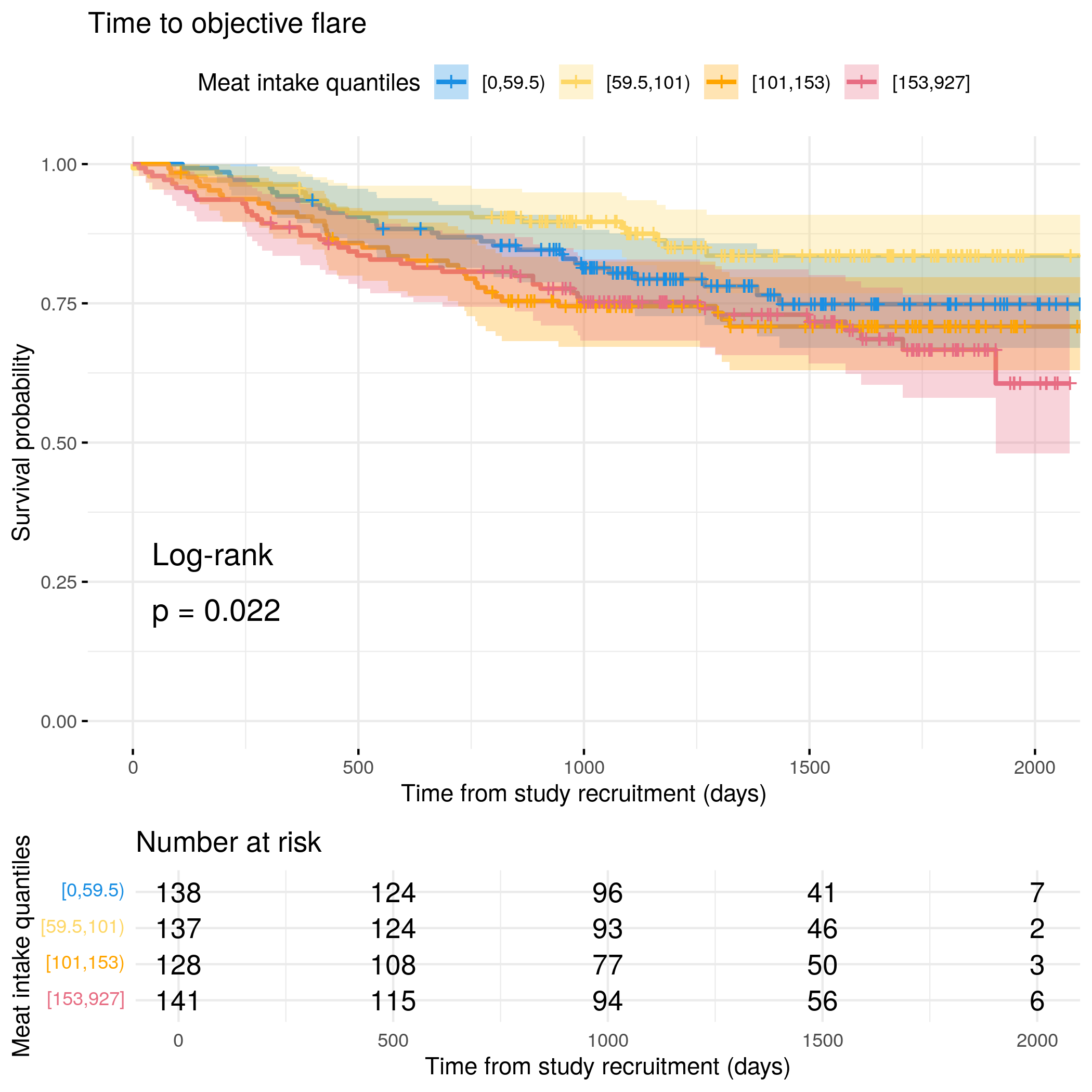
# Run survival analysis using utility function for objective flareanalysis_result<-run_survival_analysis( data =flare.df, var_name ="meat_overall", outcome_time ="hardflare_time", outcome_event ="hardflare", legend_title ="Meat intake quantiles", plot_base_path ="plots/ibd/hard-flare/diet/meat_overall", break_time_by =500)# Run Cox model with categorical variablefit.me<-coxph(Surv(hardflare_time, hardflare)~Sex+cat+IMD+dqi_tot+meat_overall_cat+frailty(SiteNo), control =coxph.control(outer.max =20), data =flare.df)hrs<-rbind(hrs, broom::tidy(fit.me)|>filter(!grepl("^Sex|^cat|^IMD|^dqi_tot|^BMI|^frailty", term))|>mutate(diagnosis ="IBD", flare ="Hard")|>relocate(diagnosis, flare))# Display plot and model summaryknitr::include_graphics("plots/ibd/hard-flare/diet/meat_overall.png")
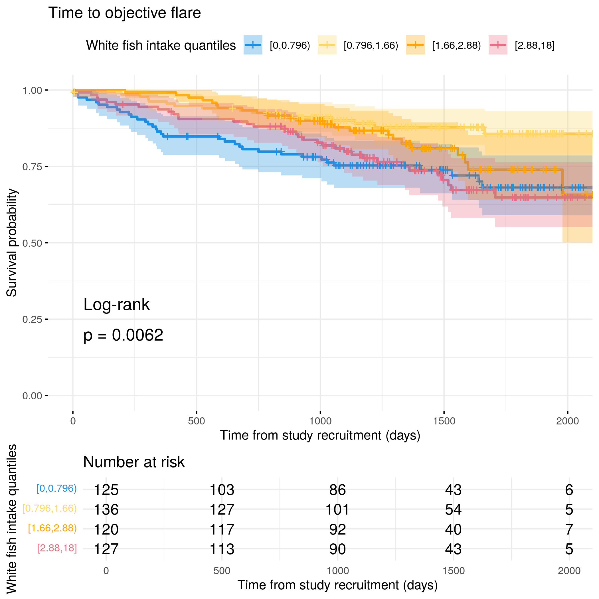
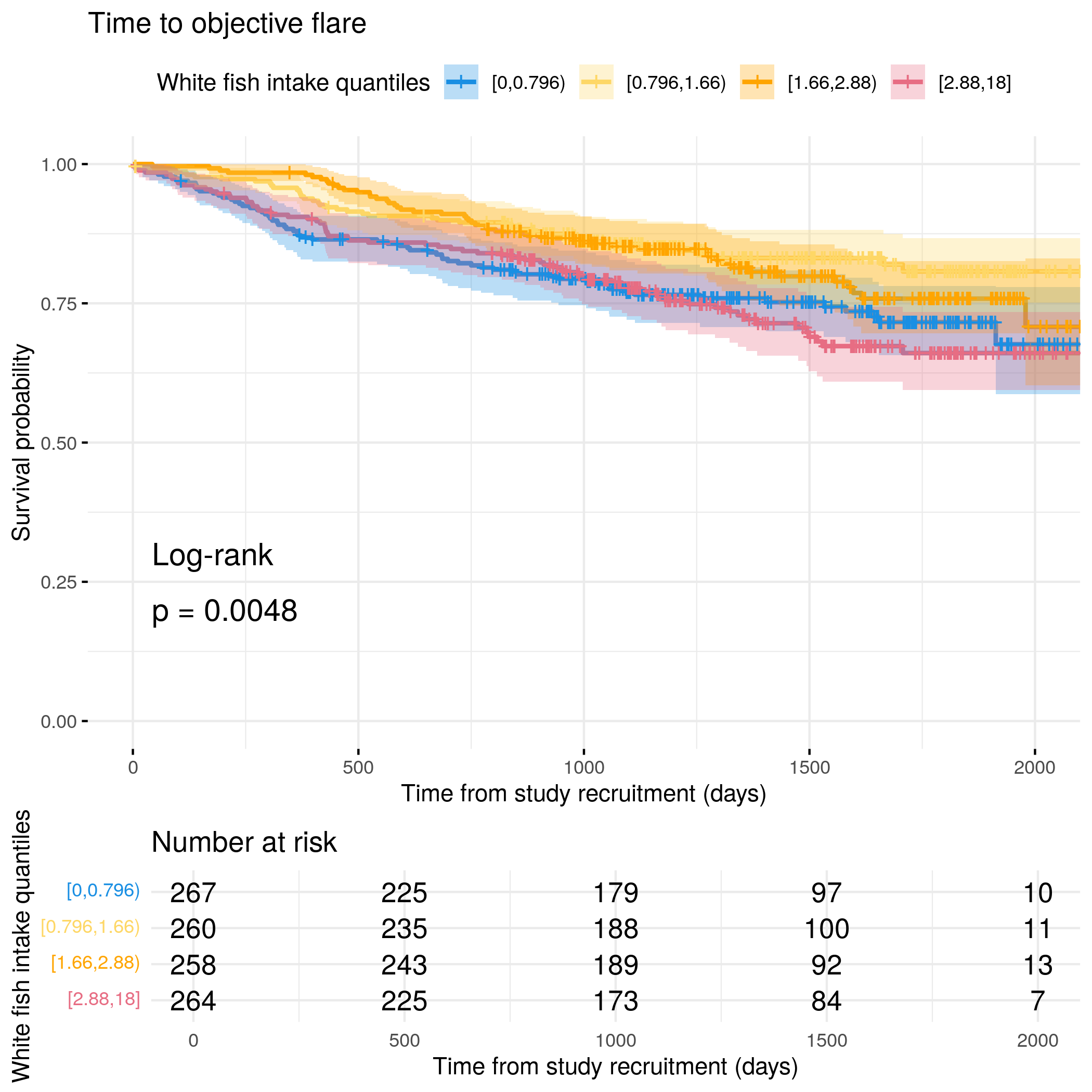
# Categorize overall fish intake by quantilesflare.cd.df<-categorize_by_quantiles(flare.cd.df, "fish_overall", reference_data =flare.df)# Run survival analysis using utility functionanalysis_result<-run_survival_analysis( data =flare.cd.df, var_name ="fish_overall", outcome_time ="softflare_time", outcome_event ="softflare", legend_title ="Fish intake quantiles", plot_base_path ="plots/cd/soft-flare/diet/fish_overall", break_time_by =200)# Save plot as RDSsaveRDS(analysis_result$plot, paste0(paths$outdir, "fish-overall-cd-soft.RDS"))# Run Cox model with categorical variablefit.me<-coxph(Surv(softflare_time, softflare)~Sex+cat+IMD+dqi_tot+fish_overall_cat+frailty(SiteNo), control =coxph.control(outer.max =20), data =flare.cd.df)hrs<-rbind(hrs, broom::tidy(fit.me)|>filter(!grepl("^Sex|^cat|^IMD|^dqi_tot|^BMI|^frailty", term))|>mutate(diagnosis ="CD", flare ="Soft")|>relocate(diagnosis, flare))# Display plot and model summaryknitr::include_graphics("plots/cd/soft-flare/diet/fish_overall.png")
# Run survival analysis using utility function for objective flareanalysis_result<-run_survival_analysis( data =flare.cd.df, var_name ="fish_overall", outcome_time ="hardflare_time", outcome_event ="hardflare", legend_title ="Fish intake quantiles", plot_base_path ="plots/cd/hard-flare/diet/fish_overall", break_time_by =500)# Save plot as RDSsaveRDS(analysis_result$plot, paste0(paths$outdir, "fish-overall-cd-hard.RDS"))# Run Cox model with categorical variablefit.me<-coxph(Surv(hardflare_time, hardflare)~Sex+cat+IMD+dqi_tot+BMI+fish_overall_cat+frailty(SiteNo), control =coxph.control(outer.max =20), data =flare.cd.df)hrs<-rbind(hrs, broom::tidy(fit.me)|>filter(!grepl("^Sex|^cat|^IMD|^dqi_tot|^BMI|^frailty", term))|>mutate(diagnosis ="CD", flare ="Hard")|>relocate(diagnosis, flare))# Display plot and model summaryknitr::include_graphics("plots/cd/hard-flare/diet/fish_overall.png")
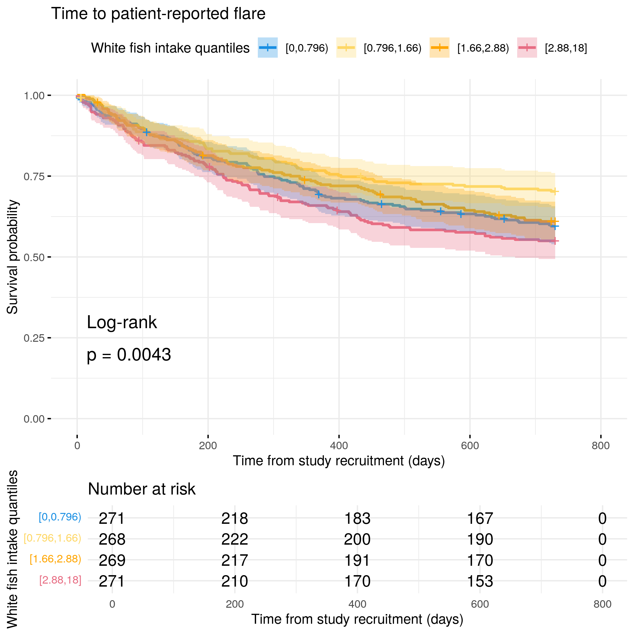
# Categorize overall fish intake by quantilesflare.uc.df<-categorize_by_quantiles(flare.uc.df, "fish_overall", reference_data =flare.df)# Run survival analysis using utility functionanalysis_result<-run_survival_analysis( data =flare.uc.df, var_name ="fish_overall", outcome_time ="softflare_time", outcome_event ="softflare", legend_title ="Fish intake quantiles", plot_base_path ="plots/uc/soft-flare/diet/fish_overall", break_time_by =200)# Save plot as RDSsaveRDS(analysis_result$plot, paste0(paths$outdir, "fish-overall-uc-soft.RDS"))# Run Cox model with categorical variablefit.me<-coxph(Surv(softflare_time, softflare)~Sex+cat+IMD+dqi_tot+BMI+fish_overall_cat+frailty(SiteNo), control =coxph.control(outer.max =20), data =flare.uc.df)hrs<-rbind(hrs, broom::tidy(fit.me)|>filter(!grepl("^Sex|^cat|^IMD|^dqi_tot|^BMI|^frailty", term))|>mutate(diagnosis ="UC", flare ="Soft")|>relocate(diagnosis, flare))# Display plot and model summaryknitr::include_graphics("plots/uc/soft-flare/diet/fish_overall.png")
# Run survival analysis using utility function for objective flareanalysis_result<-run_survival_analysis( data =flare.uc.df, var_name ="fish_overall", outcome_time ="hardflare_time", outcome_event ="hardflare", legend_title ="Fish intake quantiles", plot_base_path ="plots/uc/hard-flare/diet/fish_overall", break_time_by =500)# Save plot as RDSsaveRDS(analysis_result$plot, paste0(paths$outdir, "fish-overall-uc-hard.RDS"))# Run Cox model with categorical variablefit.me<-coxph(Surv(hardflare_time, hardflare)~Sex+cat+IMD+dqi_tot+BMI+fish_overall_cat+frailty(SiteNo), control =coxph.control(outer.max =20), data =flare.uc.df)hrs<-rbind(hrs, broom::tidy(fit.me)|>filter(!grepl("^Sex|^cat|^IMD|^dqi_tot|^BMI|^frailty", term))|>mutate(diagnosis ="UC", flare ="Hard")|>relocate(diagnosis, flare))# Display plot and model summaryknitr::include_graphics("plots/uc/hard-flare/diet/fish_overall.png")
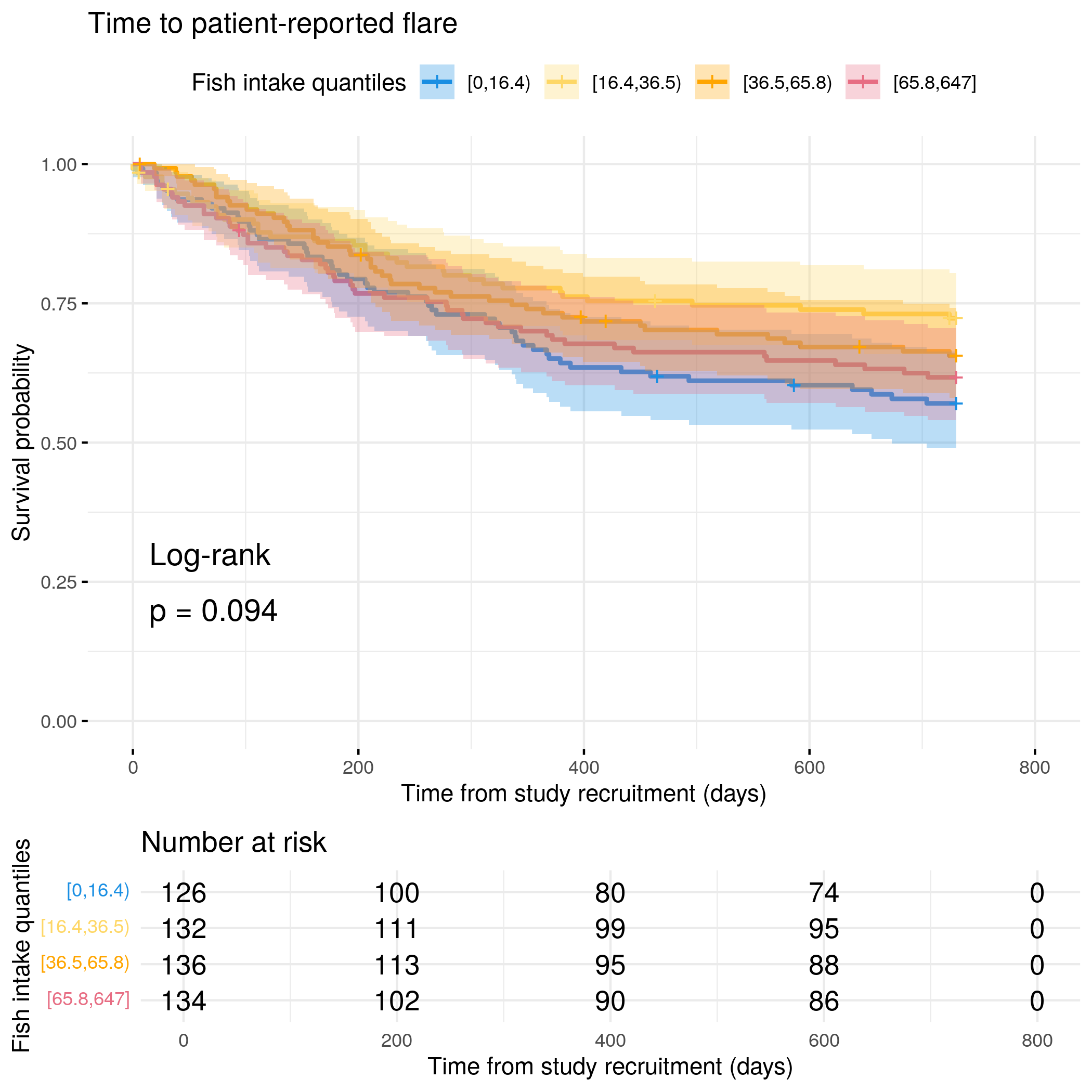
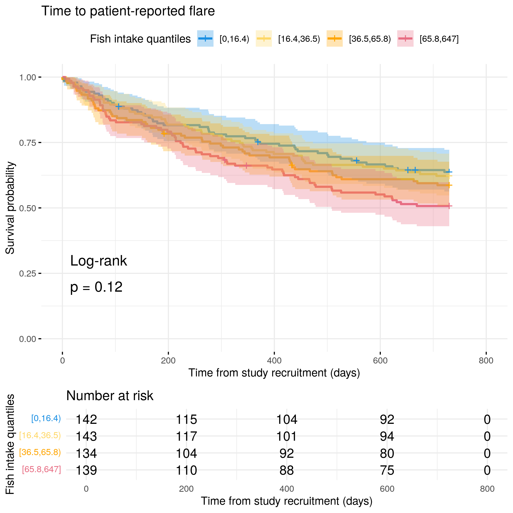
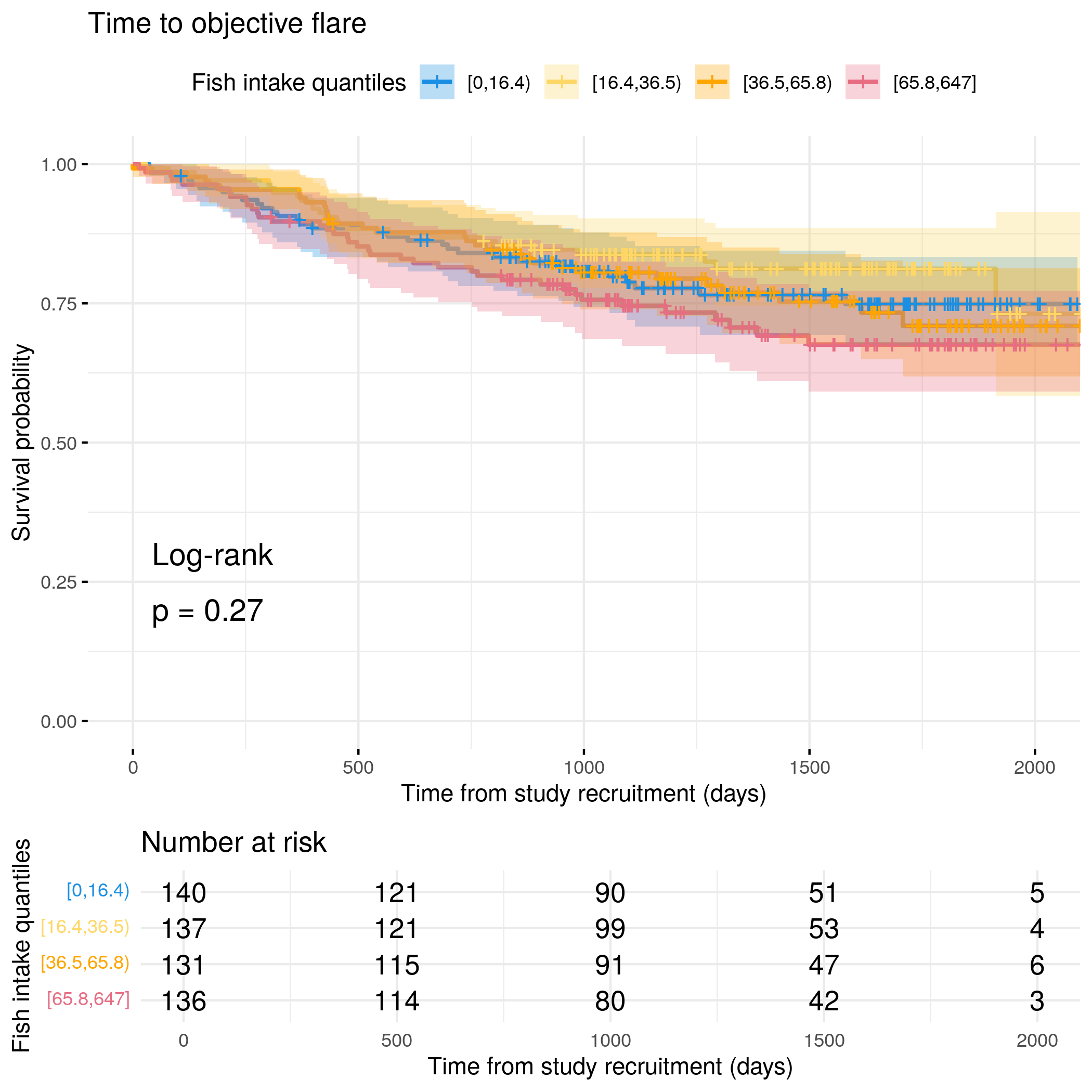
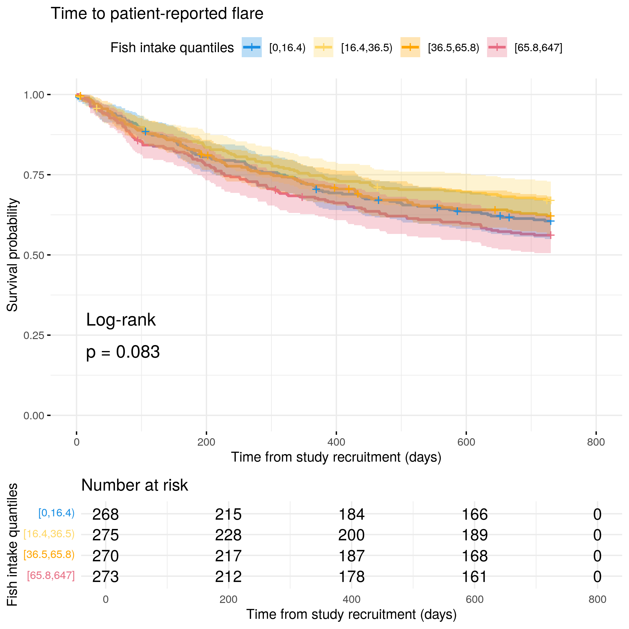
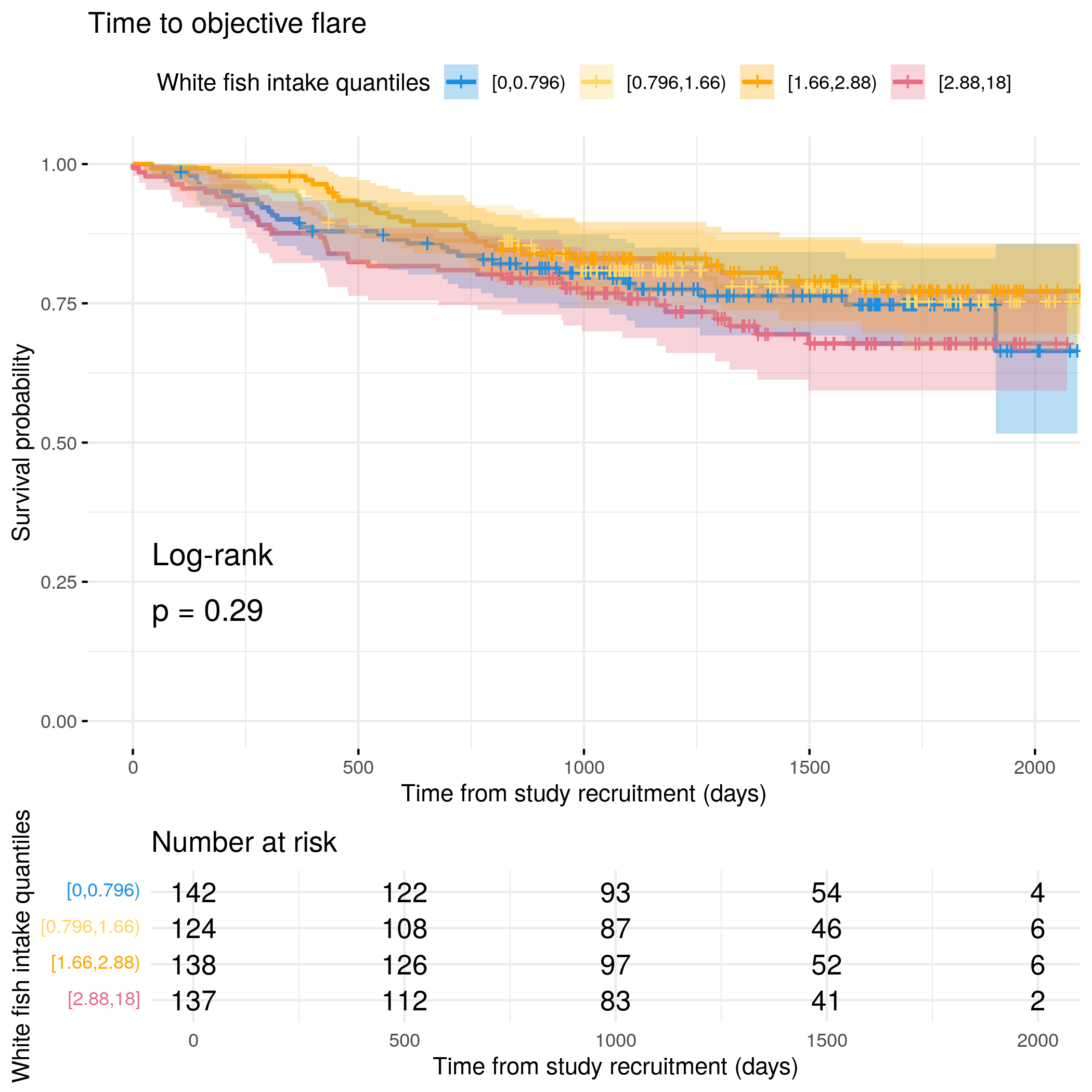
# Categorize overall fish intake by quantilesflare.df<-categorize_by_quantiles(flare.df, "fish_overall", reference_data =flare.df)# Run survival analysis using utility functionanalysis_result<-run_survival_analysis( data =flare.df, var_name ="fish_overall", outcome_time ="softflare_time", outcome_event ="softflare", legend_title ="Fish intake quantiles", plot_base_path ="plots/ibd/soft-flare/diet/fish_overall", break_time_by =200)# Run Cox model with categorical variablefit.me<-coxph(Surv(softflare_time, softflare)~Sex+cat+IMD+dqi_tot+BMI+fish_overall_cat+frailty(SiteNo), control =coxph.control(outer.max =20), data =flare.df)hrs<-rbind(hrs, broom::tidy(fit.me)|>filter(!grepl("^Sex|^cat|^IMD|^dqi_tot|^BMI|^frailty", term))|>mutate(diagnosis ="IBD", flare ="Soft")|>relocate(diagnosis, flare))# Display plot and model summaryknitr::include_graphics("plots/ibd/soft-flare/diet/fish_overall.png")
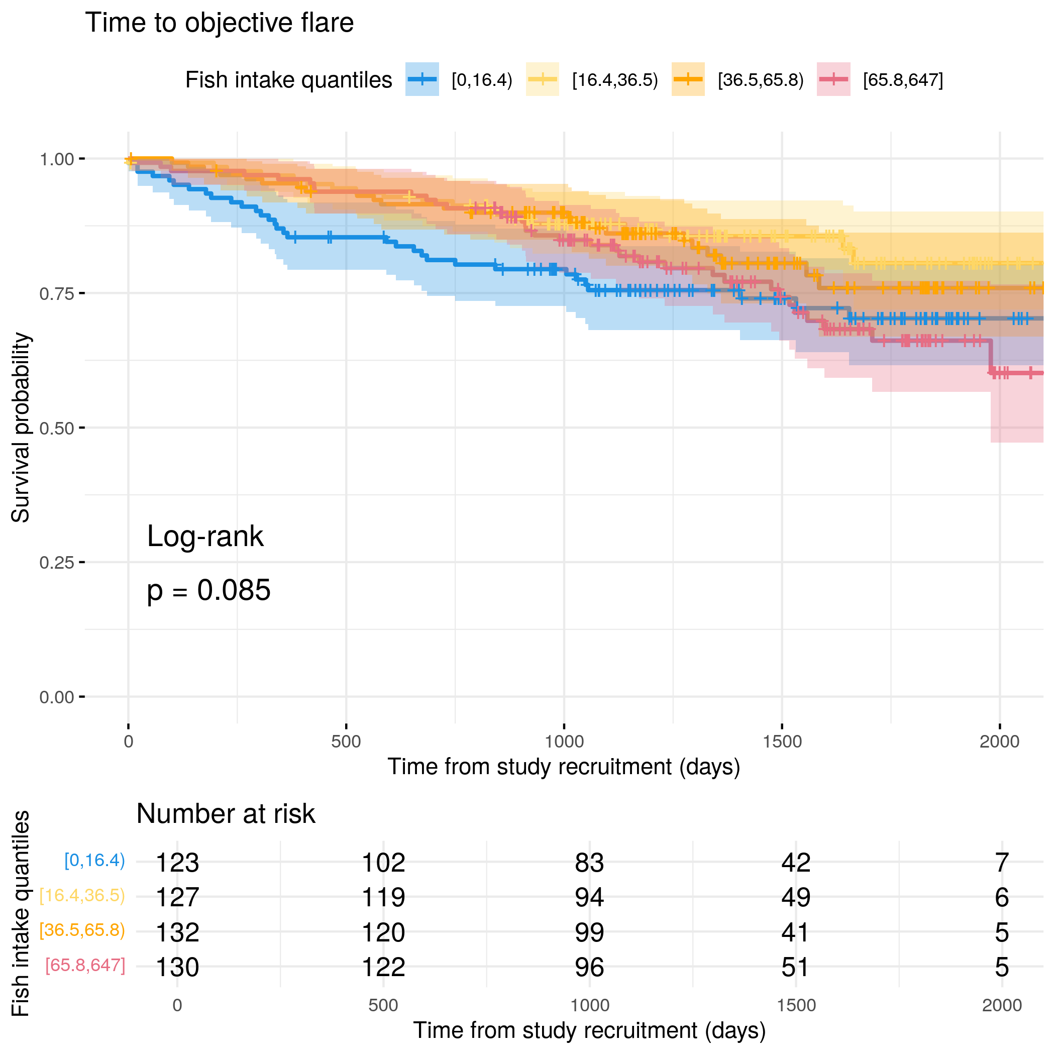
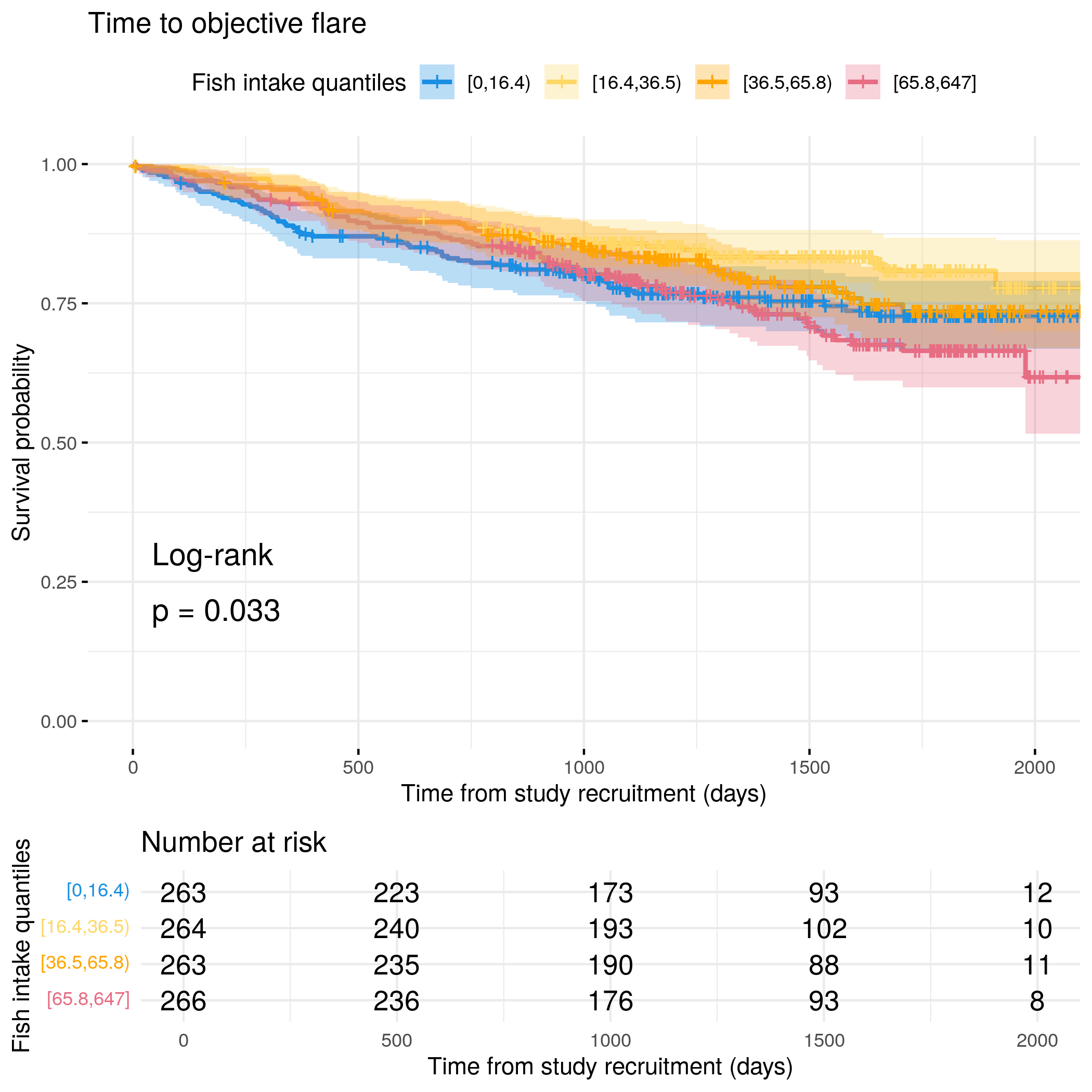
# Run survival analysis using utility function for objective flareanalysis_result<-run_survival_analysis( data =flare.df, var_name ="fish_overall", outcome_time ="hardflare_time", outcome_event ="hardflare", legend_title ="Fish intake quantiles", plot_base_path ="plots/ibd/hard-flare/diet/fish_overall", break_time_by =500)# Run Cox model with categorical variablefit.me<-coxph(Surv(hardflare_time, hardflare)~Sex+cat+IMD+dqi_tot+BMI+fish_overall_cat+frailty(SiteNo), control =coxph.control(outer.max =20), data =flare.df)hrs<-rbind(hrs, broom::tidy(fit.me)|>filter(!grepl("^Sex|^cat|^IMD|^dqi_tot|^BMI|^frailty", term))|>mutate(diagnosis ="IBD", flare ="Hard")|>relocate(diagnosis, flare))# Display plot and model summaryknitr::include_graphics("plots/ibd/hard-flare/diet/fish_overall.png")
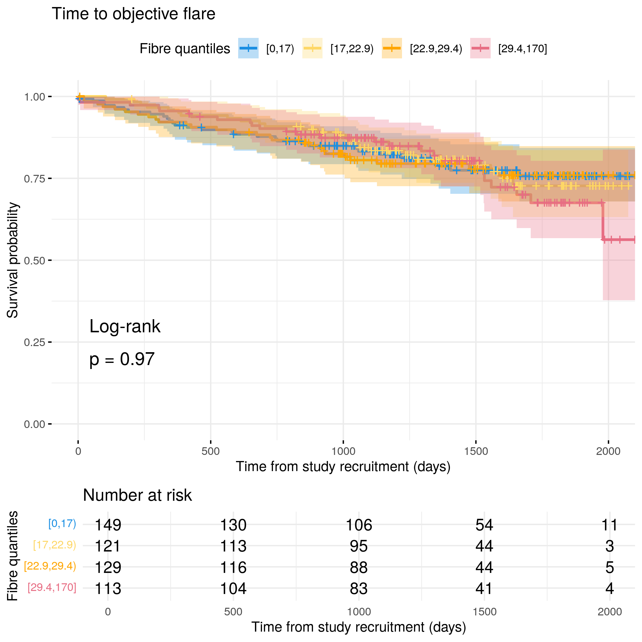
# Categorize dietary fibre by quantilesflare.cd.df<-categorize_by_quantiles(flare.cd.df, "fibre", reference_data =flare.df)# Run survival analysis using utility functionanalysis_result<-run_survival_analysis( data =flare.cd.df, var_name ="fibre", outcome_time ="softflare_time", outcome_event ="softflare", legend_title ="Fibre quantiles", plot_base_path ="plots/cd/soft-flare/diet/fibre", break_time_by =200)# Save plot as RDSsaveRDS(analysis_result$plot, paste0(paths$outdir, "fibre-cd-soft.RDS"))# Run Cox model with categorical variablefit.me<-coxph(Surv(softflare_time, softflare)~Sex+cat+IMD+dqi_tot+BMI+fibre_cat+frailty(SiteNo), control =coxph.control(outer.max =20), data =flare.cd.df)hrs<-rbind(hrs, broom::tidy(fit.me)|>filter(!grepl("^Sex|^cat|^IMD|^dqi_tot|^BMI|^frailty", term))|>mutate(diagnosis ="CD", flare ="Soft")|>relocate(diagnosis, flare))# Display plot and model summaryknitr::include_graphics("plots/cd/soft-flare/diet/fibre.png")
# Run survival analysis using utility function for objective flareanalysis_result<-run_survival_analysis( data =flare.cd.df, var_name ="fibre", outcome_time ="hardflare_time", outcome_event ="hardflare", legend_title ="Fibre quantiles", plot_base_path ="plots/cd/hard-flare/diet/fibre", break_time_by =500)# Save plot as RDSsaveRDS(analysis_result$plot, paste0(paths$outdir, "fibre-cd-hard.RDS"))# Run Cox model with categorical variablefit.me<-coxph(Surv(hardflare_time, hardflare)~Sex+cat+IMD+dqi_tot+BMI+fibre_cat+frailty(SiteNo), control =coxph.control(outer.max =20), data =flare.cd.df)hrs<-rbind(hrs, broom::tidy(fit.me)|>filter(!grepl("^Sex|^cat|^IMD|^dqi_tot|^BMI|^frailty", term))|>mutate(diagnosis ="CD", flare ="Hard")|>relocate(diagnosis, flare))# Display plot and model summaryknitr::include_graphics("plots/cd/hard-flare/diet/fibre.png")
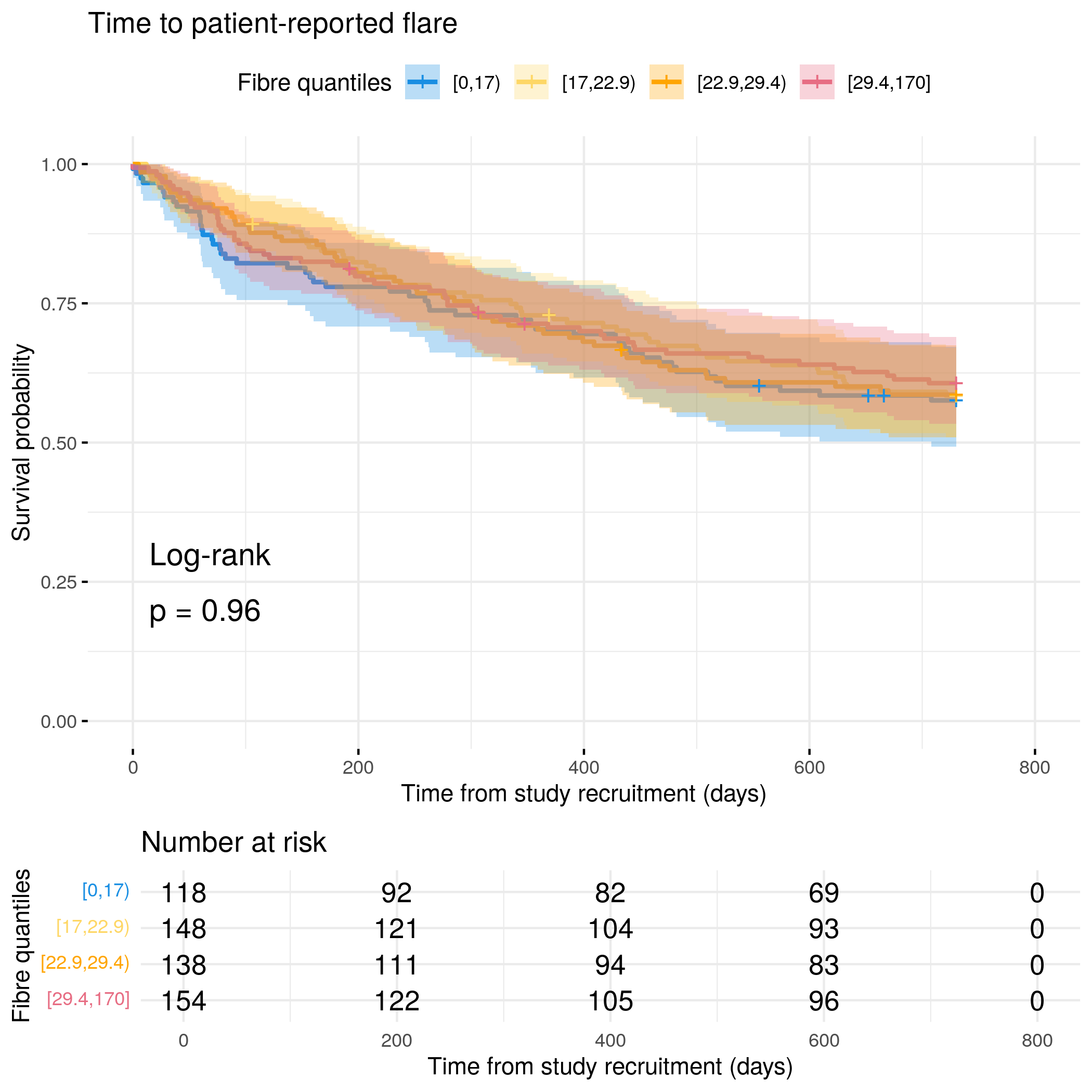
# Categorize fibre by quantilesflare.uc.df<-categorize_by_quantiles(flare.uc.df, "fibre", reference_data =flare.df)# Run survival analysis using utility functionanalysis_result<-run_survival_analysis( data =flare.uc.df, var_name ="fibre", outcome_time ="softflare_time", outcome_event ="softflare", legend_title ="Fibre quantiles", plot_base_path ="plots/uc/soft-flare/diet/fibre", break_time_by =200)# Save plot as RDSsaveRDS(analysis_result$plot, paste0(paths$outdir, "fibre-uc-soft.RDS"))# Run Cox model with categorical variablefit.me<-coxph(Surv(softflare_time, softflare)~Sex+cat+IMD+dqi_tot+BMI+fibre_cat+frailty(SiteNo), control =coxph.control(outer.max =20), data =flare.uc.df)hrs<-rbind(hrs, broom::tidy(fit.me)|>filter(!grepl("^Sex|^cat|^IMD|^dqi_tot|^BMI|^frailty", term))|>mutate(diagnosis ="UC", flare ="Soft")|>relocate(diagnosis, flare))# Display plot and model summaryknitr::include_graphics("plots/uc/soft-flare/diet/fibre.png")
# Run survival analysis using utility function for objective flareanalysis_result<-run_survival_analysis( data =flare.uc.df, var_name ="fibre", outcome_time ="hardflare_time", outcome_event ="hardflare", legend_title ="Fibre quantiles", plot_base_path ="plots/uc/hard-flare/diet/fibre", break_time_by =500)# Save plot as RDSsaveRDS(analysis_result$plot, paste0(paths$outdir, "fibre-uc-hard.RDS"))# Run Cox model with categorical variablefit.me<-coxph(Surv(hardflare_time, hardflare)~Sex+cat+IMD+dqi_tot+BMI+fibre_cat+frailty(SiteNo), control =coxph.control(outer.max =20), data =flare.uc.df)hrs<-rbind(hrs, broom::tidy(fit.me)|>filter(!grepl("^Sex|^cat|^IMD|^dqi_tot|^BMI|^frailty", term))|>mutate(diagnosis ="UC", flare ="Hard")|>relocate(diagnosis, flare))# Display plot and model summaryknitr::include_graphics("plots/uc/hard-flare/diet/fibre.png")
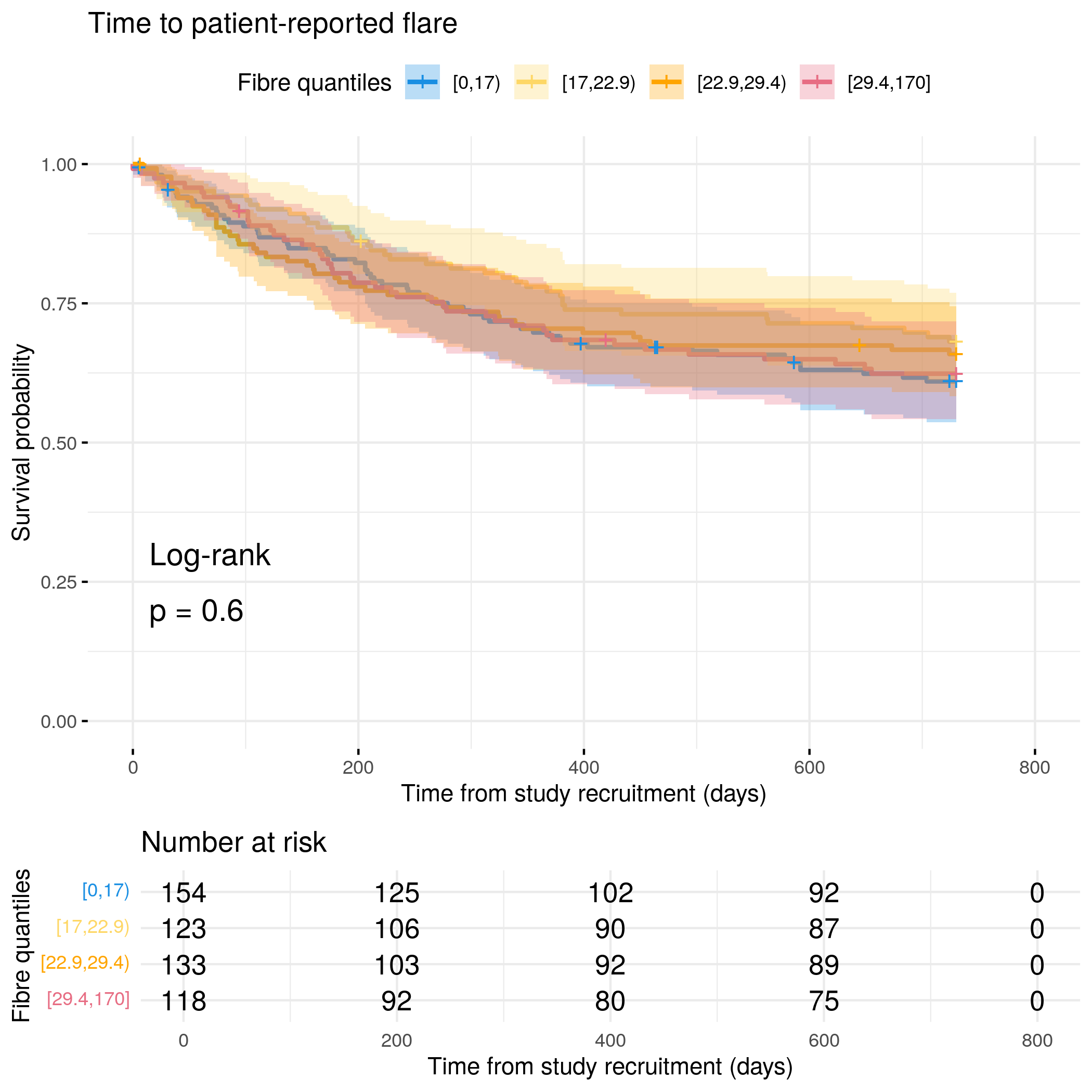
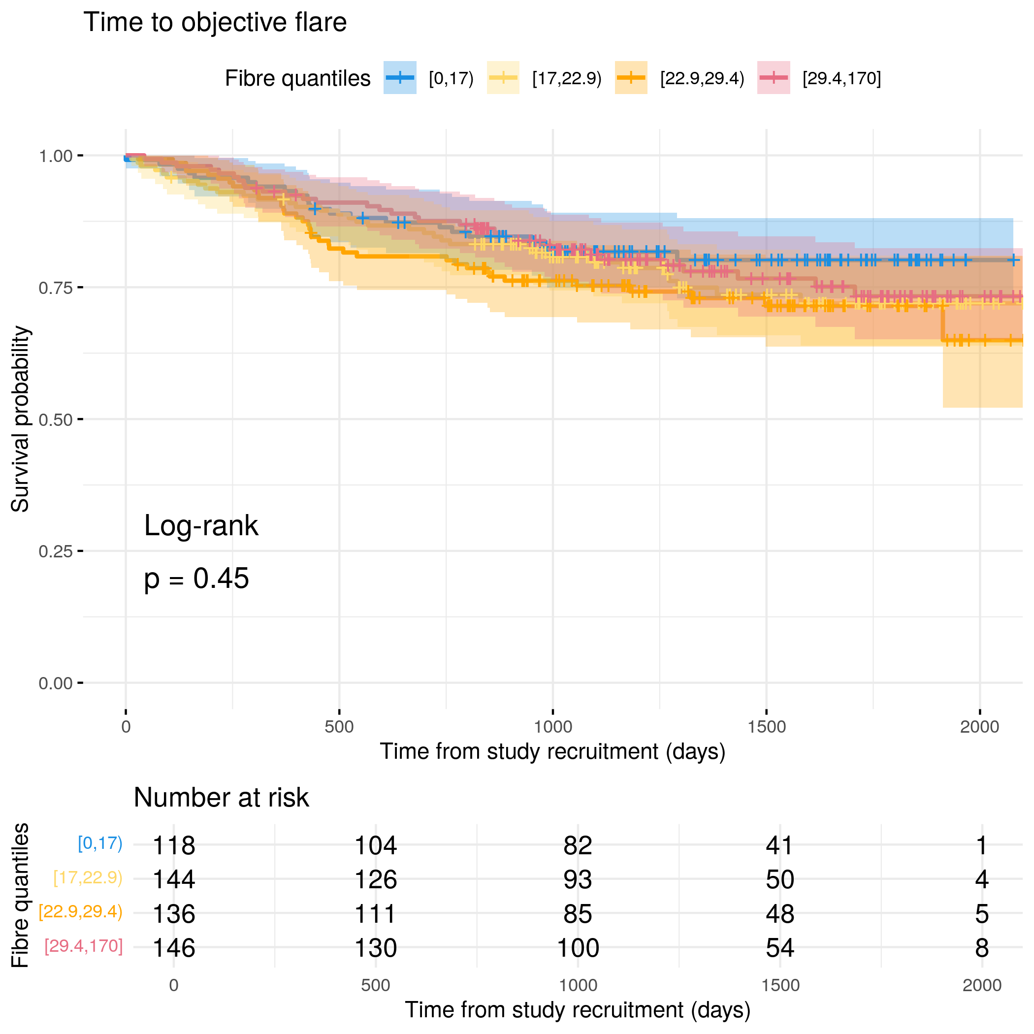
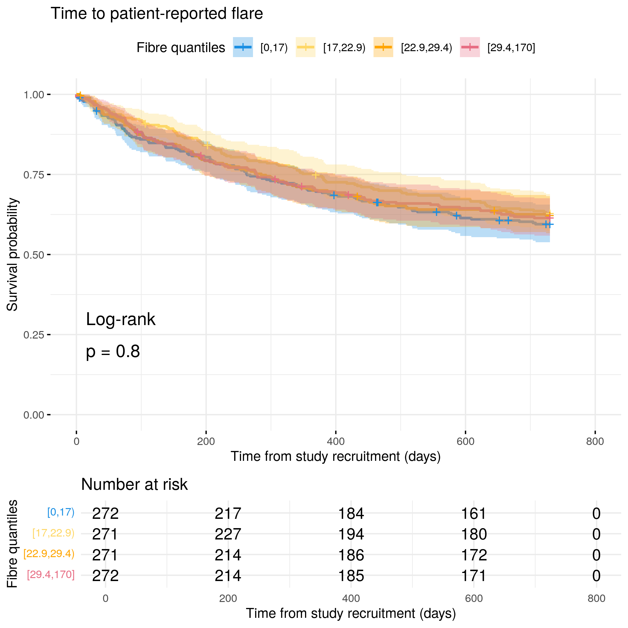
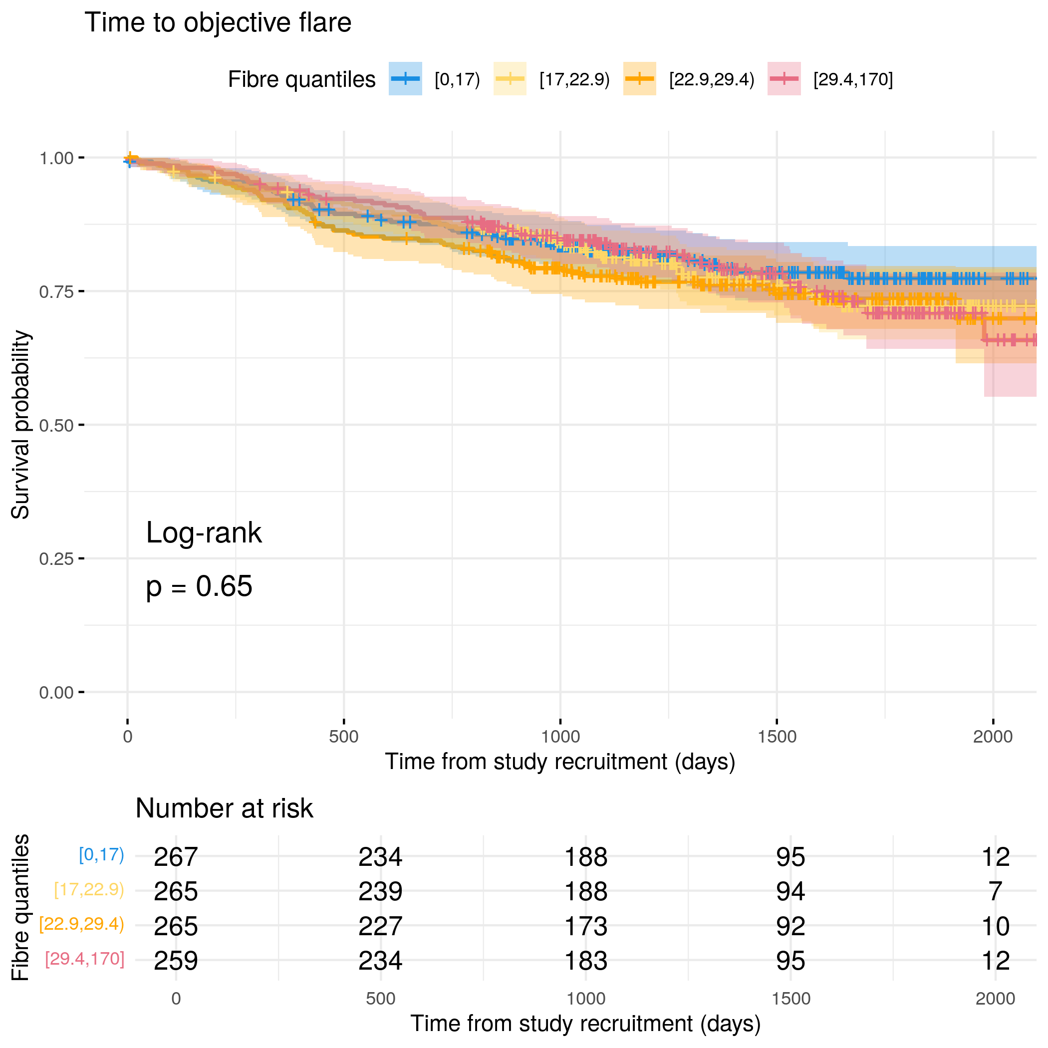
# Categorize dietary fibre by quantilesflare.df<-categorize_by_quantiles(flare.df, "fibre", reference_data =flare.df)# Run survival analysis using utility functionanalysis_result<-run_survival_analysis( data =flare.df, var_name ="fibre", outcome_time ="softflare_time", outcome_event ="softflare", legend_title ="Fibre quantiles", plot_base_path ="plots/ibd/soft-flare/diet/fibre", break_time_by =200)# Run Cox model with categorical variablefit.me<-coxph(Surv(softflare_time, softflare)~Sex+cat+IMD+dqi_tot+BMI+fibre_cat+frailty(SiteNo), control =coxph.control(outer.max =20), data =flare.df)hrs<-rbind(hrs, broom::tidy(fit.me)|>filter(!grepl("^Sex|^cat|^IMD|^dqi_tot|^BMI|^frailty", term))|>mutate(diagnosis ="IBD", flare ="Soft")|>relocate(diagnosis, flare))# Display plot and model summaryknitr::include_graphics("plots/ibd/soft-flare/diet/fibre.png")
# Run survival analysis using utility function for objective flareanalysis_result<-run_survival_analysis( data =flare.df, var_name ="fibre", outcome_time ="hardflare_time", outcome_event ="hardflare", legend_title ="Fibre quantiles", plot_base_path ="plots/ibd/hard-flare/diet/fibre", break_time_by =500)# Run Cox model with categorical variablefit.me<-coxph(Surv(hardflare_time, hardflare)~Sex+cat+IMD+dqi_tot+BMI+fibre_cat+frailty(SiteNo), control =coxph.control(outer.max =20), data =flare.df)hrs<-rbind(hrs, broom::tidy(fit.me)|>filter(!grepl("^Sex|^cat|^IMD|^dqi_tot|^BMI|^frailty", term))|>mutate(diagnosis ="IBD", flare ="Hard")|>relocate(diagnosis, flare))# Display plot and model summaryknitr::include_graphics("plots/ibd/hard-flare/diet/fibre.png")
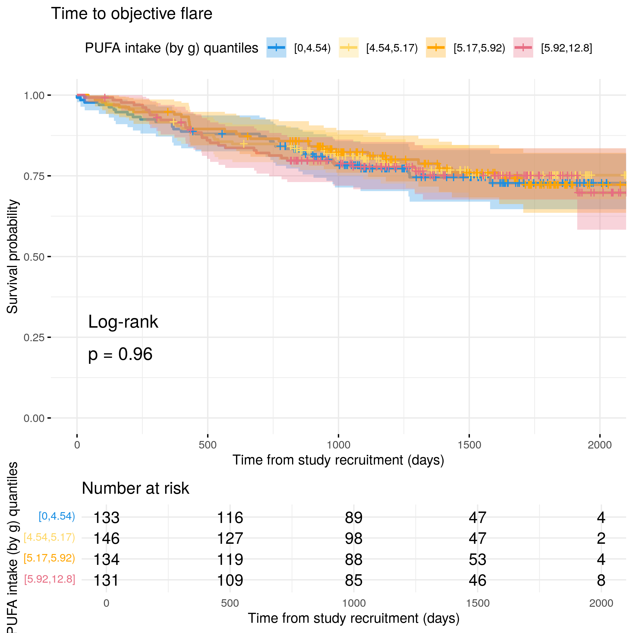
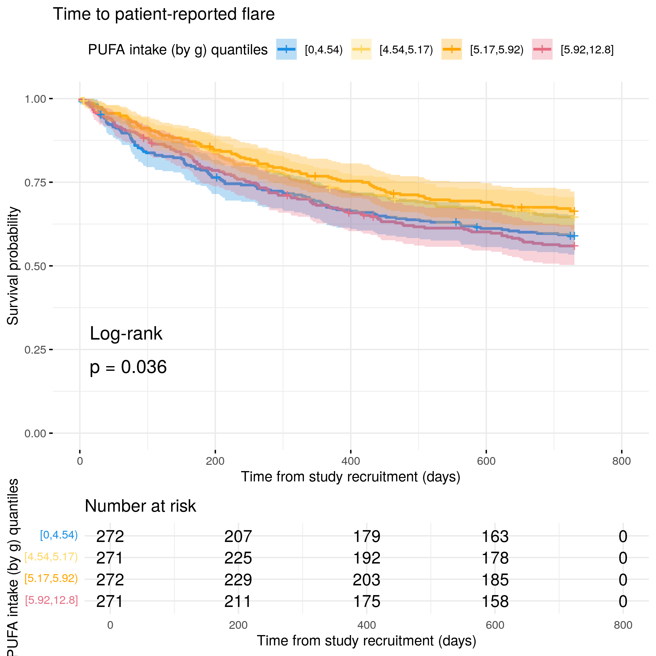
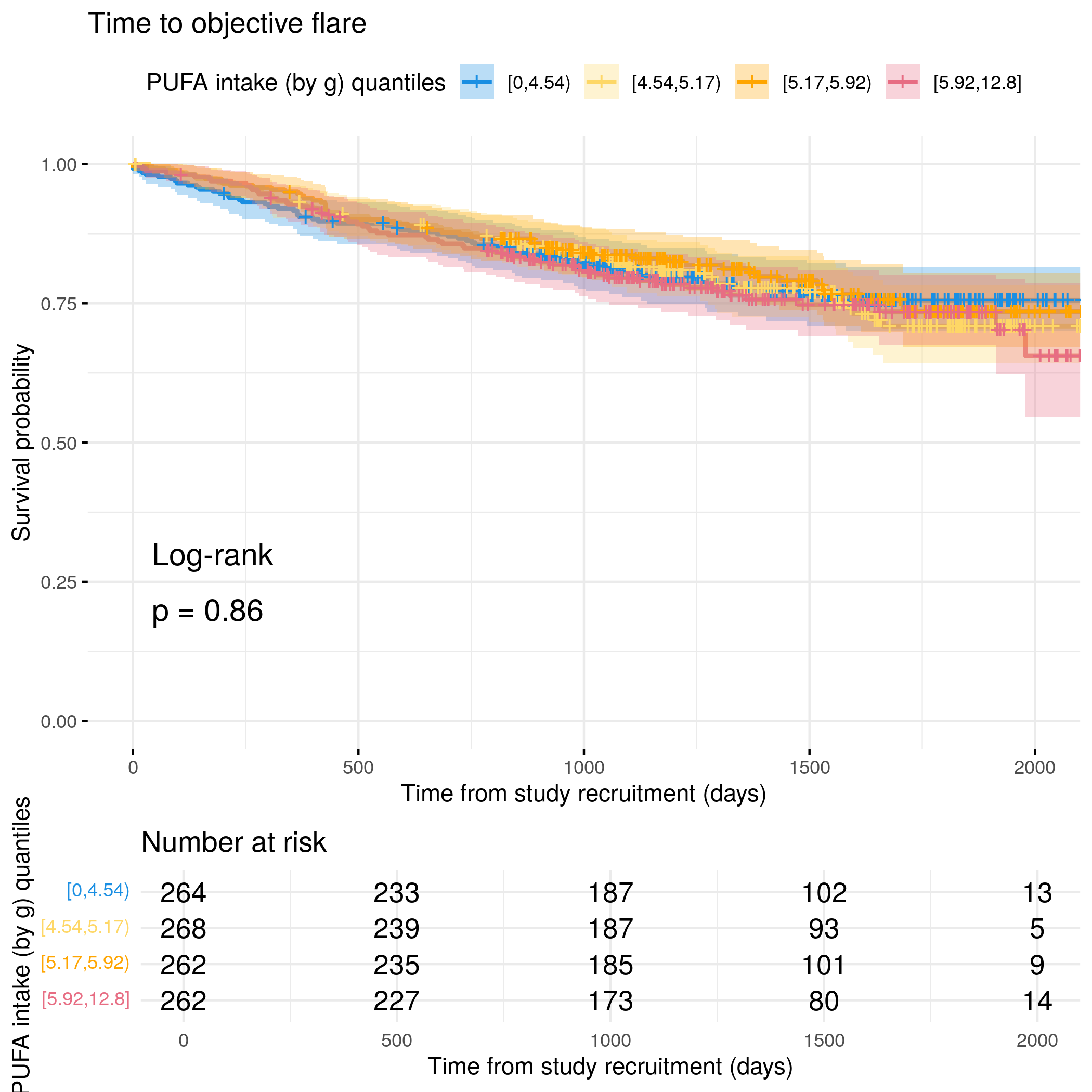
The SAP states n-6 PUFAs will be investigated. However, the FFQ data extract lists PUFA collectively, presumably describing both n-3 and n-6 PUFAs. For now, these data will be used.
# Categorize PUFA by quantilesflare.cd.df<-categorize_by_quantiles(flare.cd.df, "PUFA_percEng", reference_data =flare.df)# Run survival analysis using utility functionanalysis_result<-run_survival_analysis( data =flare.cd.df, var_name ="PUFA_percEng", outcome_time ="softflare_time", outcome_event ="softflare", legend_title ="PUFA intake (by g) quantiles", plot_base_path ="plots/cd/soft-flare/diet/pufa", break_time_by =200)# Save plot as RDSsaveRDS(analysis_result$plot, paste0(paths$outdir, "pufa-cd-soft.RDS"))# Run Cox model with categorical variablefit.me<-coxph(Surv(softflare_time, softflare)~Sex+cat+IMD+PUFA_percEng_cat+frailty(SiteNo), control =coxph.control(outer.max =20), data =flare.cd.df)hrs<-rbind(hrs, broom::tidy(fit.me)|>filter(!grepl("^Sex|^cat|^IMD|^dqi_tot|^BMI|^frailty", term))|>mutate(diagnosis ="CD", flare ="Soft")|>relocate(diagnosis, flare))# Display plot and model summaryknitr::include_graphics("plots/cd/soft-flare/diet/pufa.png")
# Run survival analysis using utility function for objective flareanalysis_result<-run_survival_analysis( data =flare.cd.df, var_name ="PUFA_percEng", outcome_time ="hardflare_time", outcome_event ="hardflare", legend_title ="PUFA intake (by g) quantiles", plot_base_path ="plots/cd/hard-flare/diet/pufa", break_time_by =500)# Save plot as RDSsaveRDS(analysis_result$plot, paste0(paths$outdir, "pufa-cd-hard.RDS"))# Run Cox model with categorical variablefit.me<-coxph(Surv(hardflare_time, hardflare)~Sex+cat+IMD+dqi_tot+BMI+PUFA_percEng_cat+frailty(SiteNo), control =coxph.control(outer.max =20), data =flare.cd.df)hrs<-rbind(hrs, broom::tidy(fit.me)|>filter(!grepl("^Sex|^cat|^IMD|^dqi_tot|^BMI|^frailty", term))|>mutate(diagnosis ="CD", flare ="Hard")|>relocate(diagnosis, flare))# Display plot and model summaryknitr::include_graphics("plots/cd/hard-flare/diet/pufa.png")
# Categorize PUFA by quantilesflare.uc.df<-categorize_by_quantiles(flare.uc.df, "PUFA_percEng", reference_data =flare.df)# Run survival analysis using utility functionanalysis_result<-run_survival_analysis( data =flare.uc.df, var_name ="PUFA_percEng", outcome_time ="softflare_time", outcome_event ="softflare", legend_title ="PUFA intake (by g) quantiles", plot_base_path ="plots/uc/soft-flare/diet/pufa", break_time_by =200)# Save plot as RDSsaveRDS(analysis_result$plot, paste0(paths$outdir, "pufa-uc-soft.RDS"))# Run Cox model with categorical variablefit.me<-coxph(Surv(softflare_time, softflare)~Sex+cat+IMD+dqi_tot+BMI+PUFA_percEng_cat+frailty(SiteNo), control =coxph.control(outer.max =20), data =flare.uc.df)hrs<-rbind(hrs, broom::tidy(fit.me)|>filter(!grepl("^Sex|^cat|^IMD|^dqi_tot|^BMI|^frailty", term))|>mutate(diagnosis ="UC", flare ="Soft")|>relocate(diagnosis, flare))# Display plot and model summaryknitr::include_graphics("plots/uc/soft-flare/diet/pufa.png")
# Run survival analysis using utility function for objective flareanalysis_result<-run_survival_analysis( data =flare.uc.df, var_name ="PUFA_percEng", outcome_time ="hardflare_time", outcome_event ="hardflare", legend_title ="PUFA intake (by g) quantiles", plot_base_path ="plots/uc/hard-flare/diet/pufa", break_time_by =500)# Save plot as RDSsaveRDS(analysis_result$plot, paste0(paths$outdir, "pufa-uc-hard.RDS"))# Run Cox model with categorical variablefit.me<-coxph(Surv(hardflare_time, hardflare)~Sex+cat+IMD+dqi_tot+BMI+PUFA_percEng_cat+frailty(SiteNo), control =coxph.control(outer.max =20), data =flare.uc.df)hrs<-rbind(hrs, broom::tidy(fit.me)|>filter(!grepl("^Sex|^cat|^IMD|^dqi_tot|^BMI|^frailty", term))|>mutate(diagnosis ="UC", flare ="Hard")|>relocate(diagnosis, flare))# Display plot and model summaryknitr::include_graphics("plots/uc/hard-flare/diet/pufa.png")
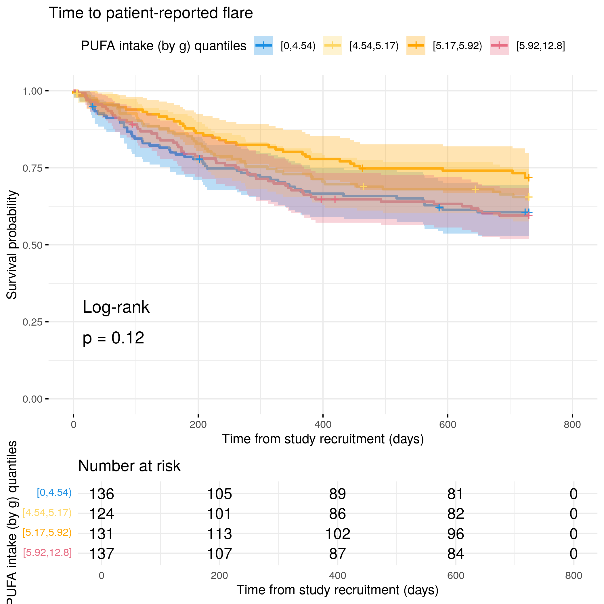
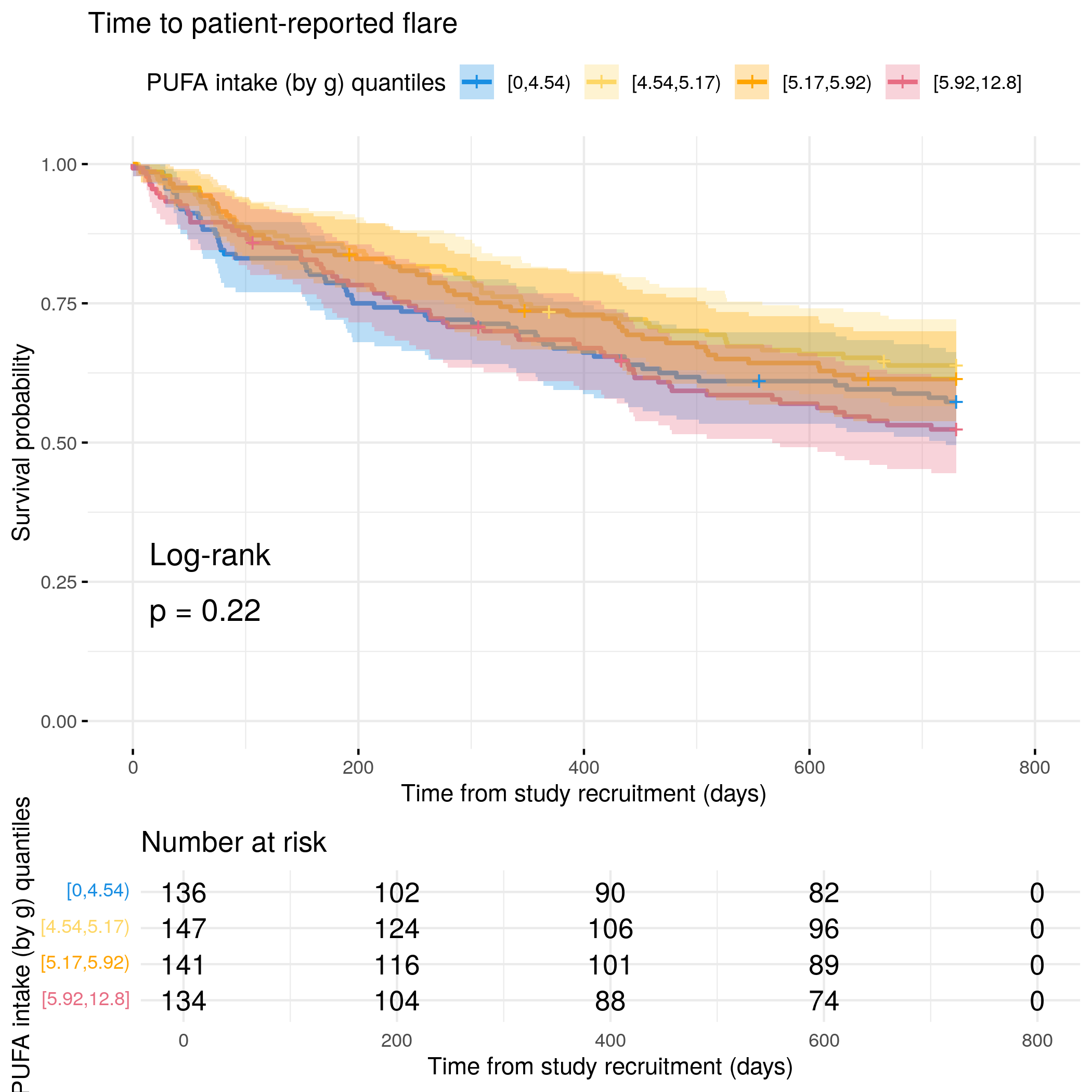
# Categorize PUFA by quantilesflare.df<-categorize_by_quantiles(flare.df, "PUFA_percEng", reference_data =flare.df)# Run survival analysis using utility functionanalysis_result<-run_survival_analysis( data =flare.df, var_name ="PUFA_percEng", outcome_time ="softflare_time", outcome_event ="softflare", legend_title ="PUFA intake (by g) quantiles", plot_base_path ="plots/ibd/soft-flare/diet/pufa", break_time_by =200)# Run Cox model with categorical variablefit.me<-coxph(Surv(softflare_time, softflare)~Sex+cat+IMD+dqi_tot+BMI+PUFA_percEng_cat+frailty(SiteNo), control =coxph.control(outer.max =20), data =flare.df)hrs<-rbind(hrs, broom::tidy(fit.me)|>filter(!grepl("^Sex|^cat|^IMD|^dqi_tot|^BMI|^frailty", term))|>mutate(diagnosis ="IBD", flare ="Soft")|>relocate(diagnosis, flare))# Display plot and model summaryknitr::include_graphics("plots/ibd/soft-flare/diet/pufa.png")
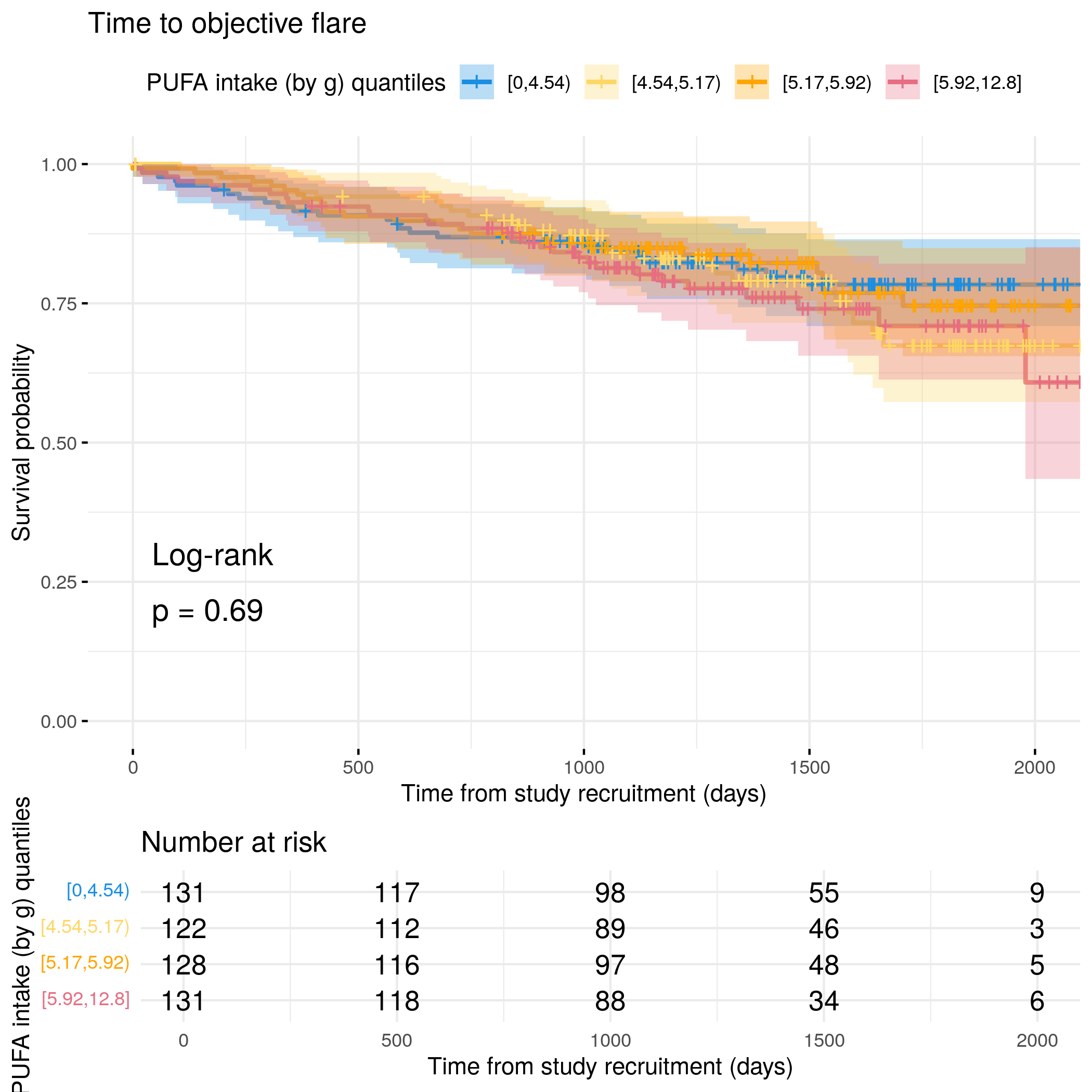
# Run survival analysis using utility function for objective flareanalysis_result<-run_survival_analysis( data =flare.df, var_name ="PUFA_percEng", outcome_time ="hardflare_time", outcome_event ="hardflare", legend_title ="PUFA intake (by g) quantiles", plot_base_path ="plots/ibd/hard-flare/diet/pufa", break_time_by =500)# Run Cox model with categorical variablefit.me<-coxph(Surv(hardflare_time, hardflare)~Sex+cat+IMD+dqi_tot+BMI+PUFA_percEng_cat+frailty(SiteNo), control =coxph.control(outer.max =20), data =flare.df)hrs<-rbind(hrs, broom::tidy(fit.me)|>filter(!grepl("^Sex|^cat|^IMD|^dqi_tot|^BMI|^frailty", term))|>mutate(diagnosis ="IBD", flare ="Hard")|>relocate(diagnosis, flare))# Display plot and model summaryknitr::include_graphics("plots/ibd/hard-flare/diet/pufa.png")
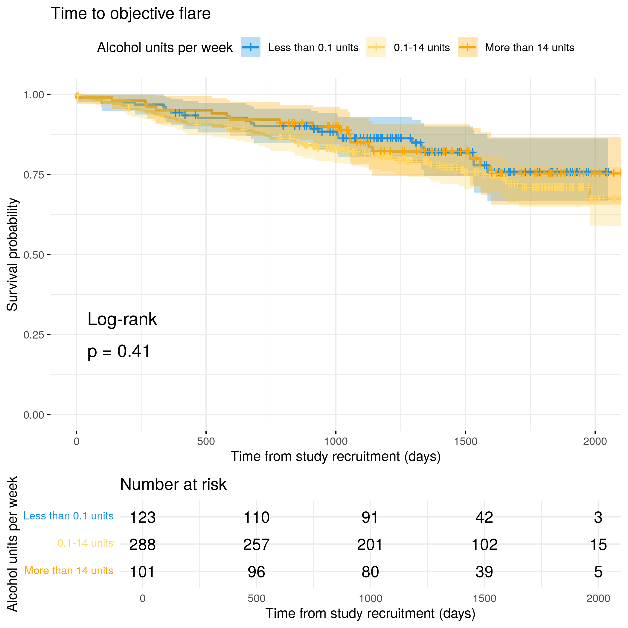
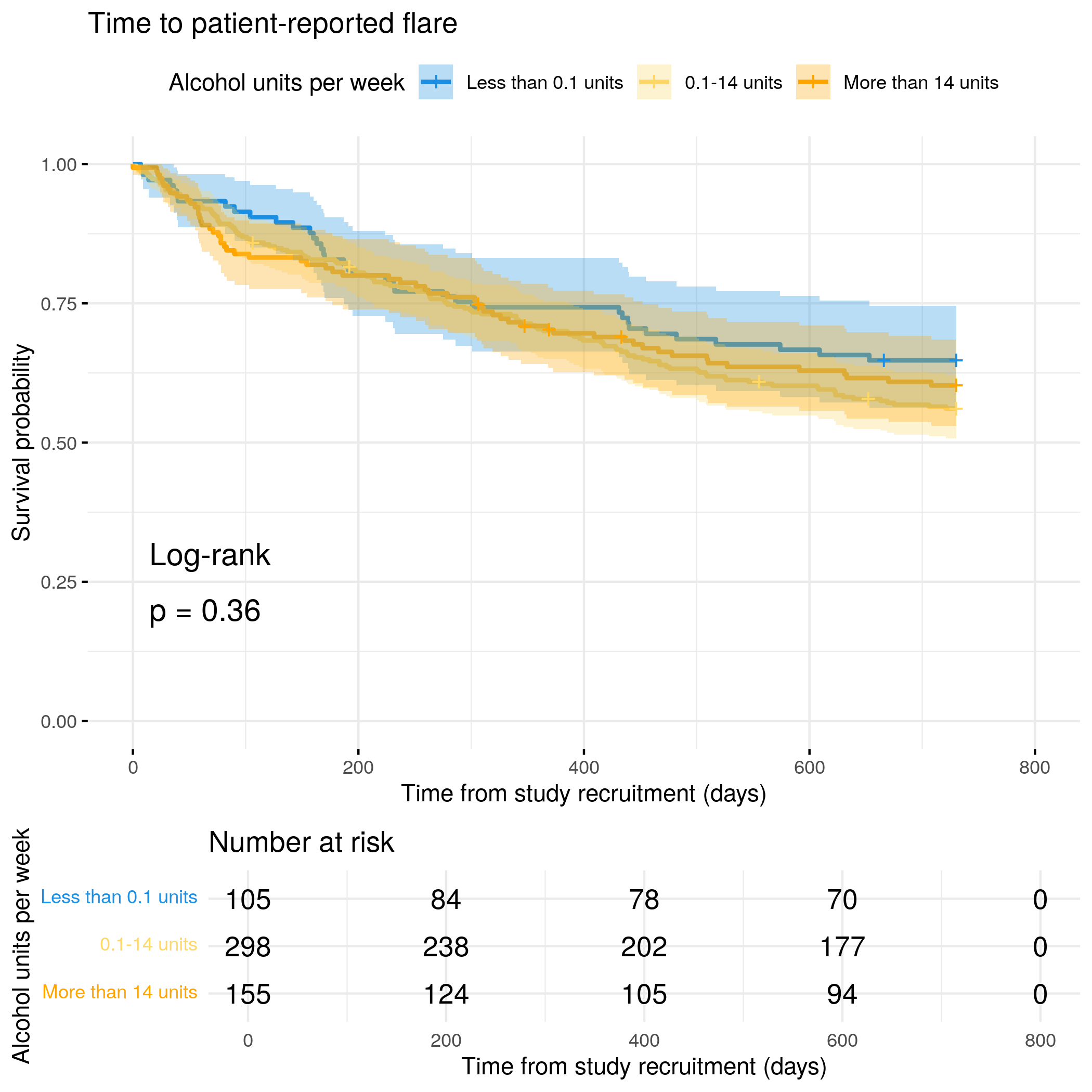
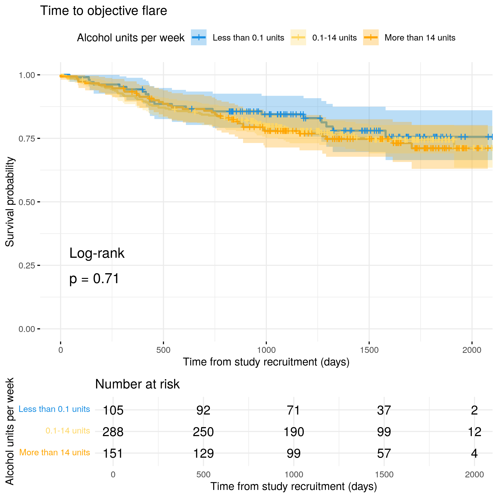
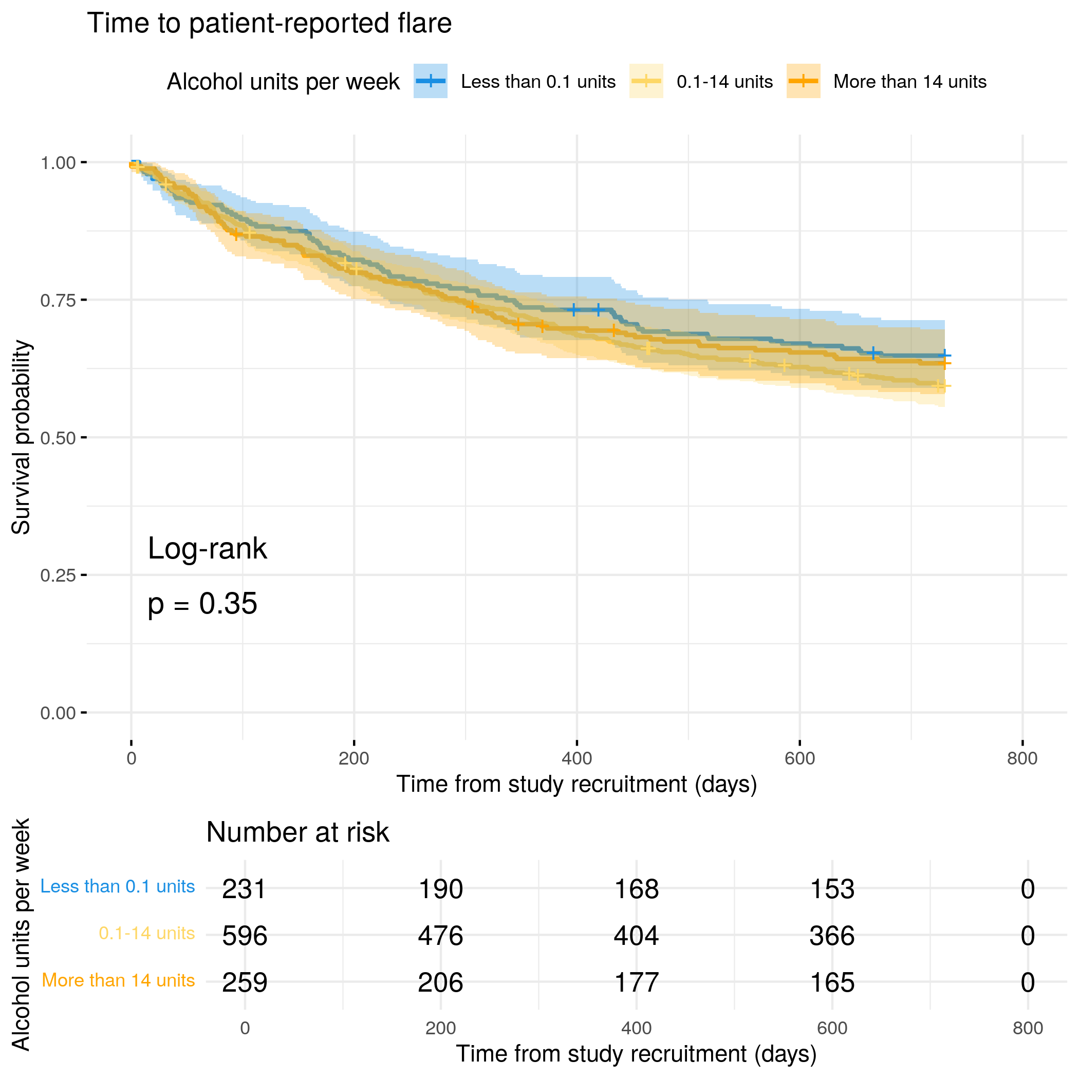
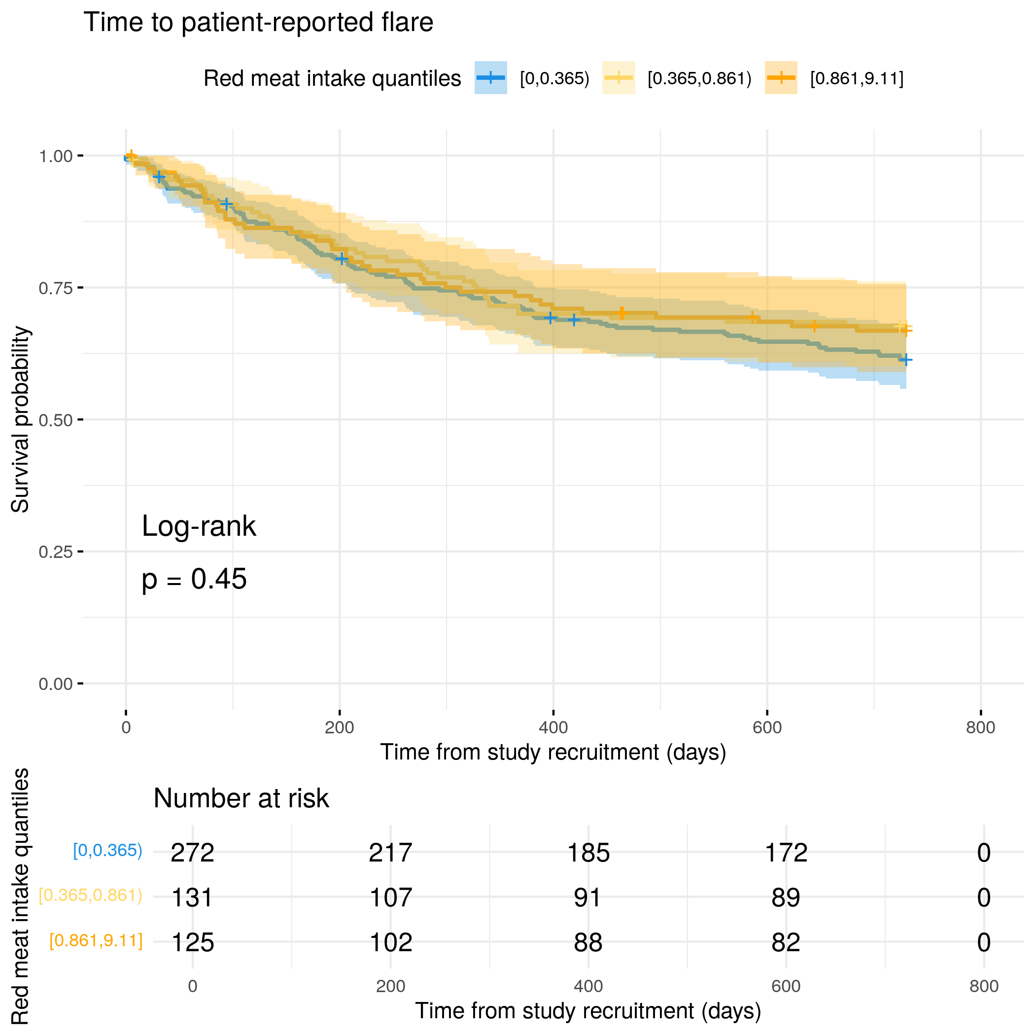
levels(flare.cd.df$weekly_units_cat)<-c("Less than 0.1 units", "0.1-14 units", "More than 14 units")# Run survival analysis using utility functionanalysis_result<-run_survival_analysis( data =flare.cd.df, var_name ="weekly_units", outcome_time ="softflare_time", outcome_event ="softflare", legend_title ="Alcohol units per week", plot_base_path ="plots/cd/soft-flare/diet/alcohol", break_time_by =200)# Save plot as RDSsaveRDS(analysis_result$plot, paste0(paths$outdir, "alcohol-cd-soft.RDS"))# Run Cox model with categorical variablefit.me<-coxph(Surv(softflare_time, softflare)~Sex+cat+IMD+dqi_tot+weekly_units_cat+frailty(SiteNo), control =coxph.control(outer.max =20), data =flare.cd.df)hrs<-rbind(hrs, broom::tidy(fit.me)|>filter(!grepl("^Sex|^cat|^IMD|^dqi_tot|^BMI|^frailty", term))|>mutate(diagnosis ="CD", flare ="Soft")|>relocate(diagnosis, flare))# Display plot and model summaryknitr::include_graphics("plots/cd/soft-flare/diet/alcohol.png")
# Run survival analysis using utility function for objective flareanalysis_result<-run_survival_analysis( data =flare.cd.df, var_name ="weekly_units", outcome_time ="hardflare_time", outcome_event ="hardflare", legend_title ="Alcohol units per week", plot_base_path ="plots/cd/hard-flare/diet/alcohol", break_time_by =500)# Save plot as RDSsaveRDS(analysis_result$plot, paste0(paths$outdir, "alcohol-cd-hard.RDS"))# Run Cox model with categorical variablefit.me<-coxph(Surv(hardflare_time, hardflare)~Sex+cat+IMD+dqi_tot+weekly_units_cat+frailty(SiteNo), control =coxph.control(outer.max =20), data =flare.cd.df)hrs<-rbind(hrs, broom::tidy(fit.me)|>filter(!grepl("^Sex|^cat|^IMD|^dqi_tot|^BMI|^frailty", term))|>mutate(diagnosis ="CD", flare ="Hard")|>relocate(diagnosis, flare))# Display plot and model summaryknitr::include_graphics("plots/cd/hard-flare/diet/alcohol.png")
# Run survival analysis using utility functionanalysis_result<-run_survival_analysis( data =flare.uc.df, var_name ="weekly_units", outcome_time ="softflare_time", outcome_event ="softflare", legend_title ="Alcohol units per week", plot_base_path ="plots/uc/soft-flare/diet/alcohol", break_time_by =200)# Save plot as RDSsaveRDS(analysis_result$plot, paste0(paths$outdir, "alcohol-uc-soft.RDS"))# Run Cox model with categorical variablefit.me<-coxph(Surv(softflare_time, softflare)~Sex+cat+IMD+dqi_tot+weekly_units_cat+frailty(SiteNo), control =coxph.control(outer.max =20), data =flare.uc.df)hrs<-rbind(hrs, broom::tidy(fit.me)|>filter(!grepl("^Sex|^cat|^IMD|^dqi_tot|^BMI|^frailty", term))|>mutate(diagnosis ="UC", flare ="Soft")|>relocate(diagnosis, flare))# Display plot and model summaryknitr::include_graphics("plots/uc/soft-flare/diet/alcohol.png")
# Run survival analysis using utility function for objective flareanalysis_result<-run_survival_analysis( data =flare.uc.df, var_name ="weekly_units", outcome_time ="hardflare_time", outcome_event ="hardflare", legend_title ="Alcohol units per week", plot_base_path ="plots/uc/hard-flare/diet/alcohol", break_time_by =500)# Save plot as RDSsaveRDS(analysis_result$plot, paste0(paths$outdir, "alcohol-uc-hard.RDS"))# Run Cox model with categorical variablefit.me<-coxph(Surv(hardflare_time, hardflare)~Sex+cat+IMD+dqi_tot+weekly_units_cat+frailty(SiteNo), control =coxph.control(outer.max =20), data =flare.uc.df)hrs<-rbind(hrs, broom::tidy(fit.me)|>filter(!grepl("^Sex|^cat|^IMD|^dqi_tot|^BMI|^frailty", term))|>mutate(diagnosis ="UC", flare ="Hard")|>relocate(diagnosis, flare))# Display plot and model summaryknitr::include_graphics("plots/uc/hard-flare/diet/alcohol.png")
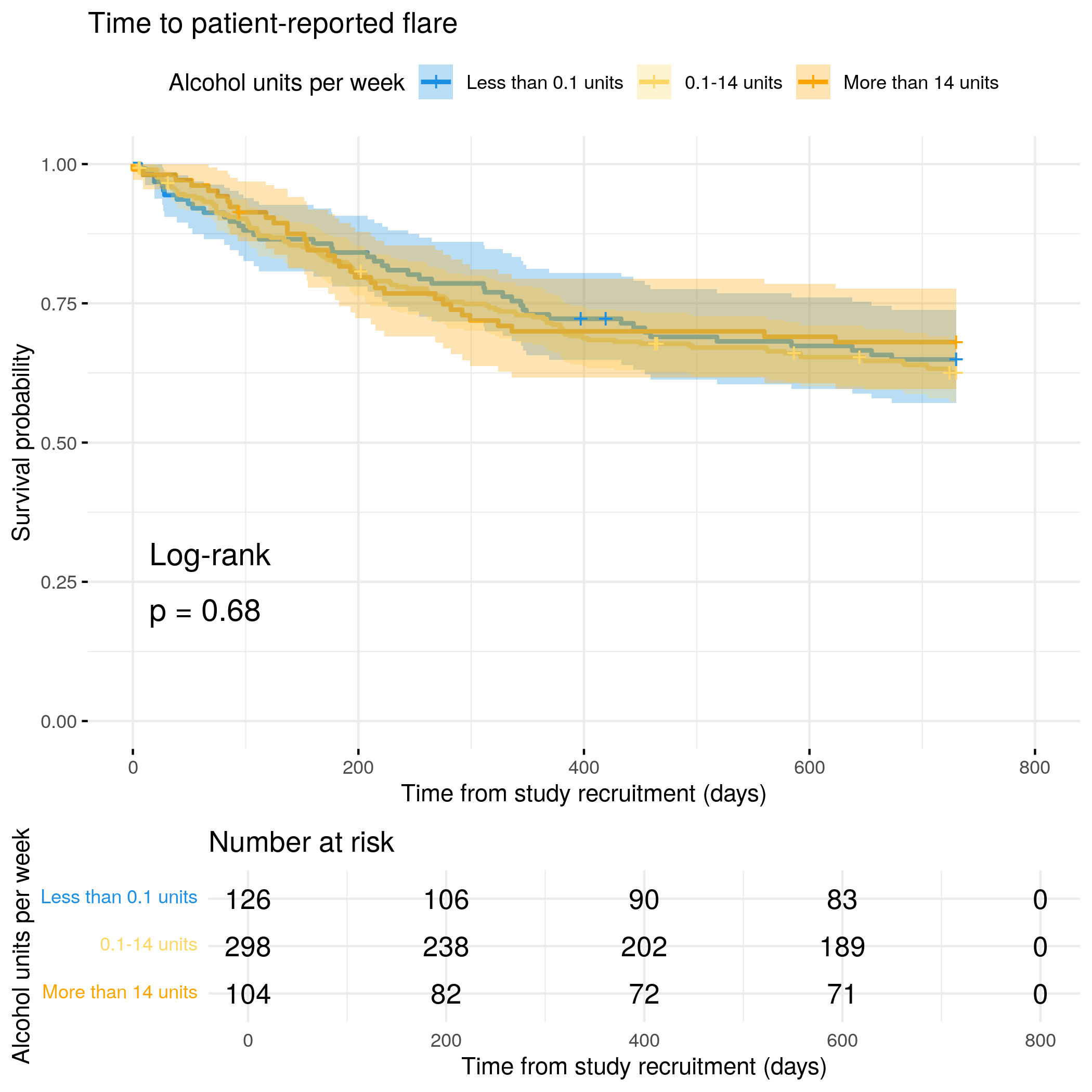
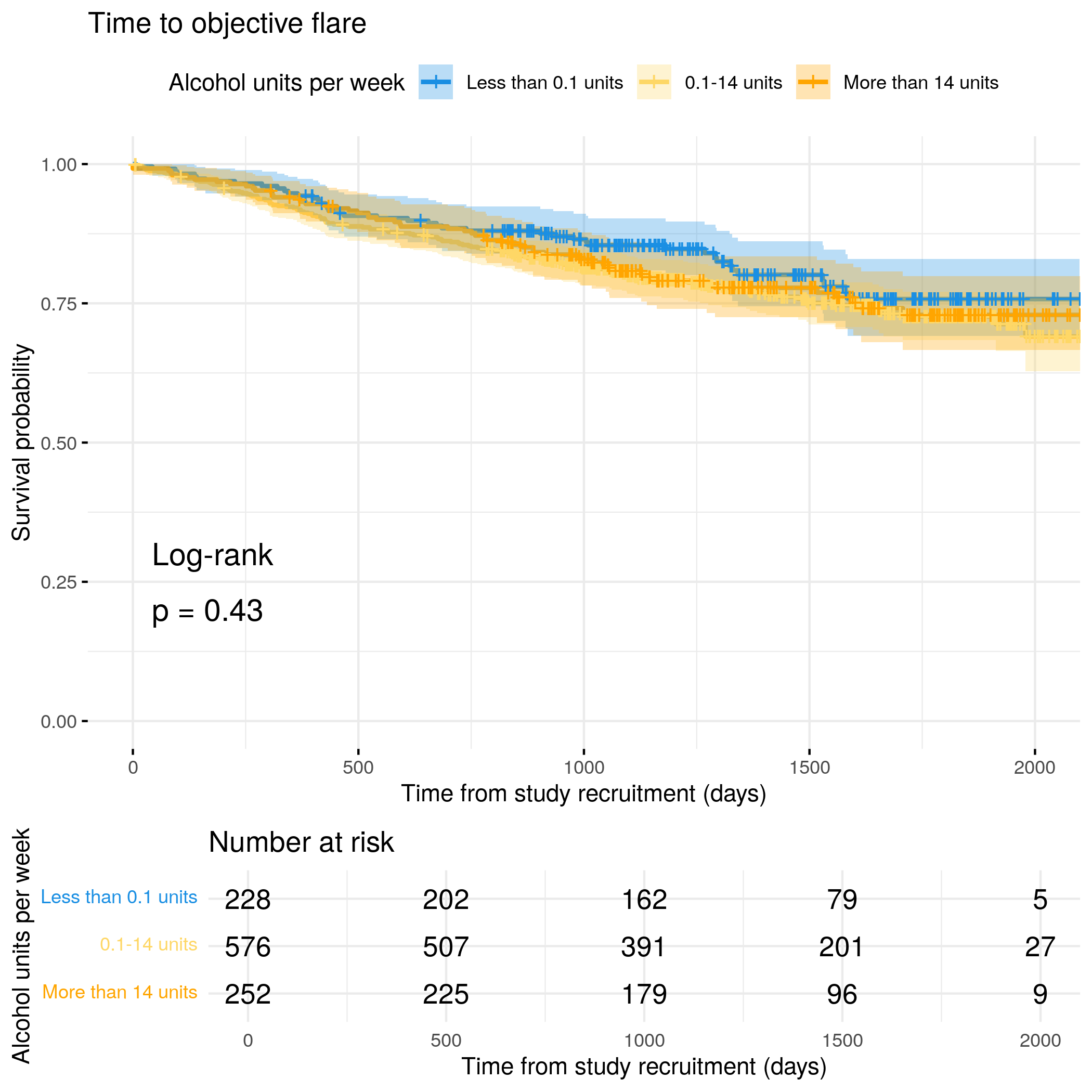
# Run survival analysis using utility functionanalysis_result<-run_survival_analysis( data =flare.df, var_name ="weekly_units", outcome_time ="softflare_time", outcome_event ="softflare", legend_title ="Alcohol units per week", plot_base_path ="plots/ibd/soft-flare/diet/alcohol", break_time_by =200)# Run Cox model with categorical variablefit.me<-coxph(Surv(softflare_time, softflare)~Sex+cat+IMD+dqi_tot+weekly_units_cat+frailty(SiteNo), control =coxph.control(outer.max =20), data =flare.df)hrs<-rbind(hrs, broom::tidy(fit.me)|>filter(!grepl("^Sex|^cat|^IMD|^dqi_tot|^BMI|^frailty", term))|>mutate(diagnosis ="IBD", flare ="Soft")|>relocate(diagnosis, flare))# Display plot and model summaryknitr::include_graphics("plots/ibd/soft-flare/diet/alcohol.png")
# Run survival analysis using utility function for objective flareanalysis_result<-run_survival_analysis( data =flare.df, var_name ="weekly_units", outcome_time ="hardflare_time", outcome_event ="hardflare", legend_title ="Alcohol units per week", plot_base_path ="plots/ibd/hard-flare/diet/alcohol", break_time_by =500)# Run Cox model with categorical variablefit.me<-coxph(Surv(hardflare_time, hardflare)~Sex+cat+IMD+dqi_tot+weekly_units_cat+frailty(SiteNo), control =coxph.control(outer.max =20), data =flare.df)hrs<-rbind(hrs, broom::tidy(fit.me)|>filter(!grepl("^Sex|^cat|^IMD|^dqi_tot|^BMI|^frailty", term))|>mutate(diagnosis ="IBD", flare ="Hard")|>relocate(diagnosis, flare))# Display plot and model summaryknitr::include_graphics("plots/ibd/hard-flare/diet/alcohol.png")
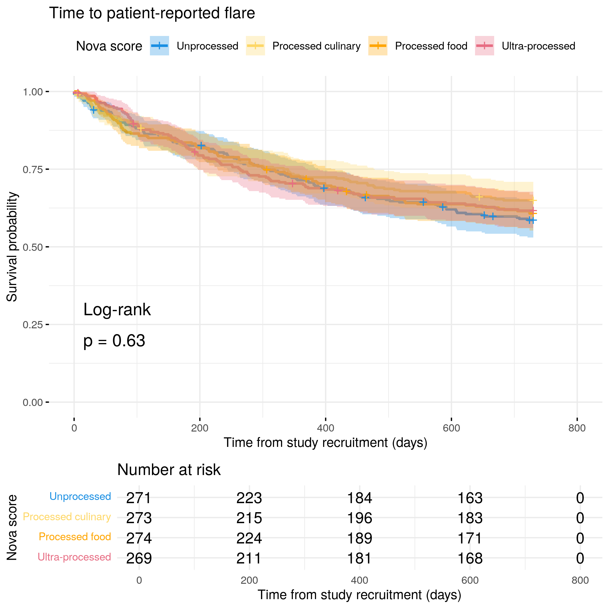
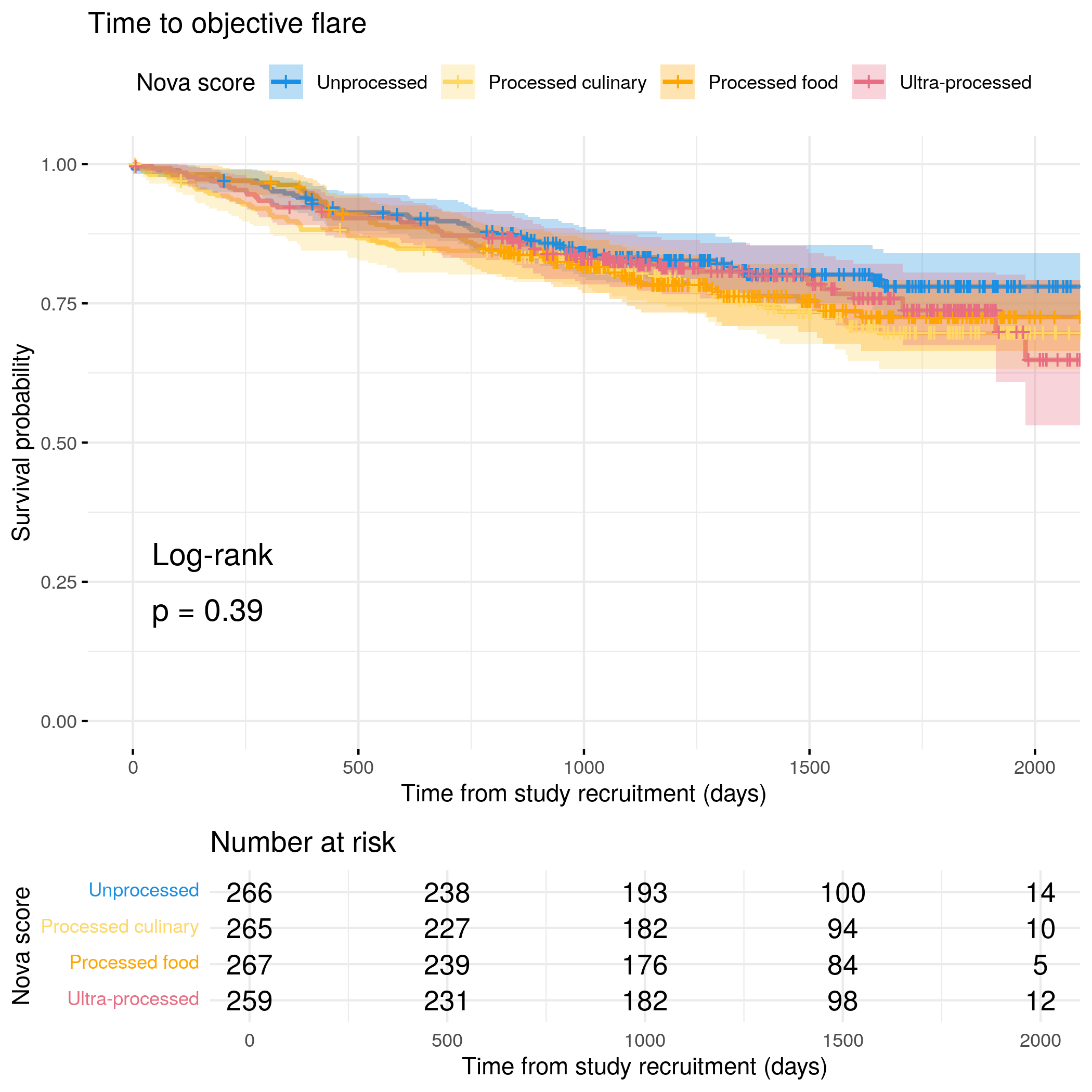
The SAP states emulsifiers (specifically lecithin) will be investigated. However, data on emulsifiers are not available in the FFQ data extract. As a proxy for emulsifiers, this report will look at ultra-processed foods via Nova scores (Monteiro et al. 2017).
# Run survival analysis using utility functionanalysis_result<-run_survival_analysis( data =flare.cd.df, var_name ="NOVAScore", outcome_time ="softflare_time", outcome_event ="softflare", legend_title ="Nova score", plot_base_path ="plots/cd/soft-flare/diet/nova", break_time_by =200)# Save plot as RDSsaveRDS(analysis_result$plot, paste0(paths$outdir, "nova-cd-soft.RDS"))# Run Cox model with categorical variablefit.me<-coxph(Surv(softflare_time, softflare)~Sex+cat+IMD+dqi_tot+BMI+NOVAScore_cat+frailty(SiteNo), control =coxph.control(outer.max =20), data =flare.cd.df)hrs<-rbind(hrs, broom::tidy(fit.me)|>filter(!grepl("^Sex|^cat|^IMD|^dqi_tot|^BMI|^frailty", term))|>mutate(diagnosis ="CD", flare ="Soft")|>relocate(diagnosis, flare))# Display plot and model summaryknitr::include_graphics("plots/cd/soft-flare/diet/nova.png")
# Run survival analysis using utility function for objective flareanalysis_result<-run_survival_analysis( data =flare.cd.df, var_name ="NOVAScore", outcome_time ="hardflare_time", outcome_event ="hardflare", legend_title ="Nova Score", plot_base_path ="plots/cd/hard-flare/diet/nova", break_time_by =500)# Save plot as RDSsaveRDS(analysis_result$plot, paste0(paths$outdir, "nova-cd-hard.RDS"))# Run Cox model with categorical variablefit.me<-coxph(Surv(hardflare_time, hardflare)~Sex+cat+IMD+dqi_tot+BMI+NOVAScore_cat+frailty(SiteNo), control =coxph.control(outer.max =20), data =flare.cd.df)hrs<-rbind(hrs, broom::tidy(fit.me)|>filter(!grepl("^Sex|^cat|^IMD|^dqi_tot|^BMI|^frailty", term))|>mutate(diagnosis ="CD", flare ="Hard")|>relocate(diagnosis, flare))# Display plot and model summaryknitr::include_graphics("plots/cd/hard-flare/diet/nova.png")
# Run survival analysis using utility functionanalysis_result<-run_survival_analysis( data =flare.uc.df, var_name ="NOVAScore", outcome_time ="softflare_time", outcome_event ="softflare", legend_title ="Nova score", plot_base_path ="plots/uc/soft-flare/diet/nova", break_time_by =200)# Save plot as RDSsaveRDS(analysis_result$plot, paste0(paths$outdir, "nova-uc-soft.RDS"))# Run Cox model with categorical variablefit.me<-coxph(Surv(softflare_time, softflare)~Sex+cat+IMD+dqi_tot+BMI+NOVAScore_cat+frailty(SiteNo), control =coxph.control(outer.max =20), data =flare.uc.df)hrs<-rbind(hrs, broom::tidy(fit.me)|>filter(!grepl("^Sex|^cat|^IMD|^dqi_tot|^BMI|^frailty", term))|>mutate(diagnosis ="UC", flare ="Soft")|>relocate(diagnosis, flare))# Display plot and model summaryknitr::include_graphics("plots/uc/soft-flare/diet/nova.png")
# Run survival analysis using utility function for objective flareanalysis_result<-run_survival_analysis( data =flare.uc.df, var_name ="NOVAScore", outcome_time ="hardflare_time", outcome_event ="hardflare", legend_title ="Nova score", plot_base_path ="plots/uc/hard-flare/diet/nova", break_time_by =500)# Save plot as RDSsaveRDS(analysis_result$plot, paste0(paths$outdir, "nova-uc-hard.RDS"))# Run Cox model with categorical variablefit.me<-coxph(Surv(hardflare_time, hardflare)~Sex+cat+IMD+dqi_tot+BMI+NOVAScore_cat+frailty(SiteNo), control =coxph.control(outer.max =20), data =flare.uc.df)hrs<-rbind(hrs, broom::tidy(fit.me)|>filter(!grepl("^Sex|^cat|^IMD|^dqi_tot|^BMI|^frailty", term))|>mutate(diagnosis ="UC", flare ="Hard")|>relocate(diagnosis, flare))# Display plot and model summaryknitr::include_graphics("plots/uc/hard-flare/diet/nova.png")
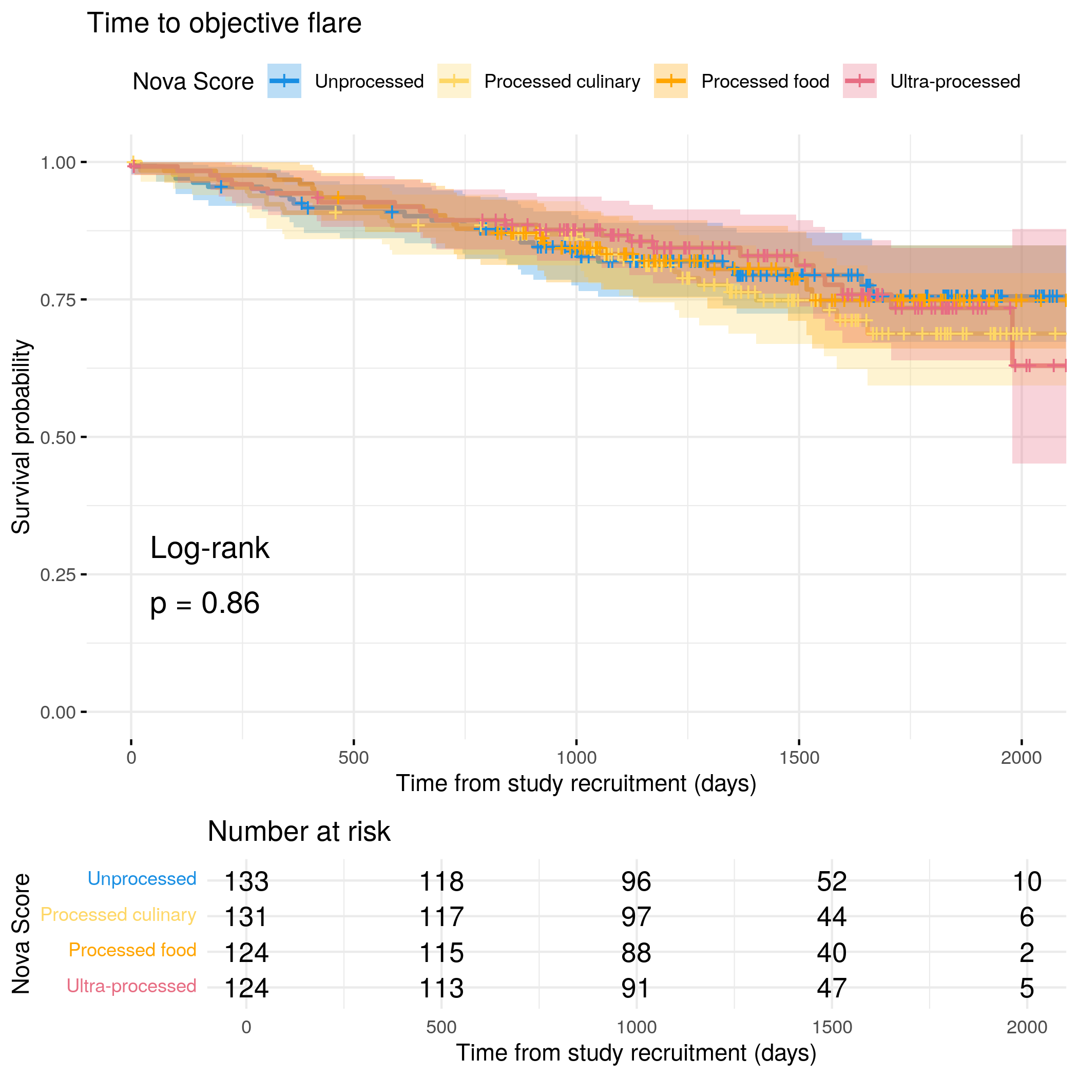
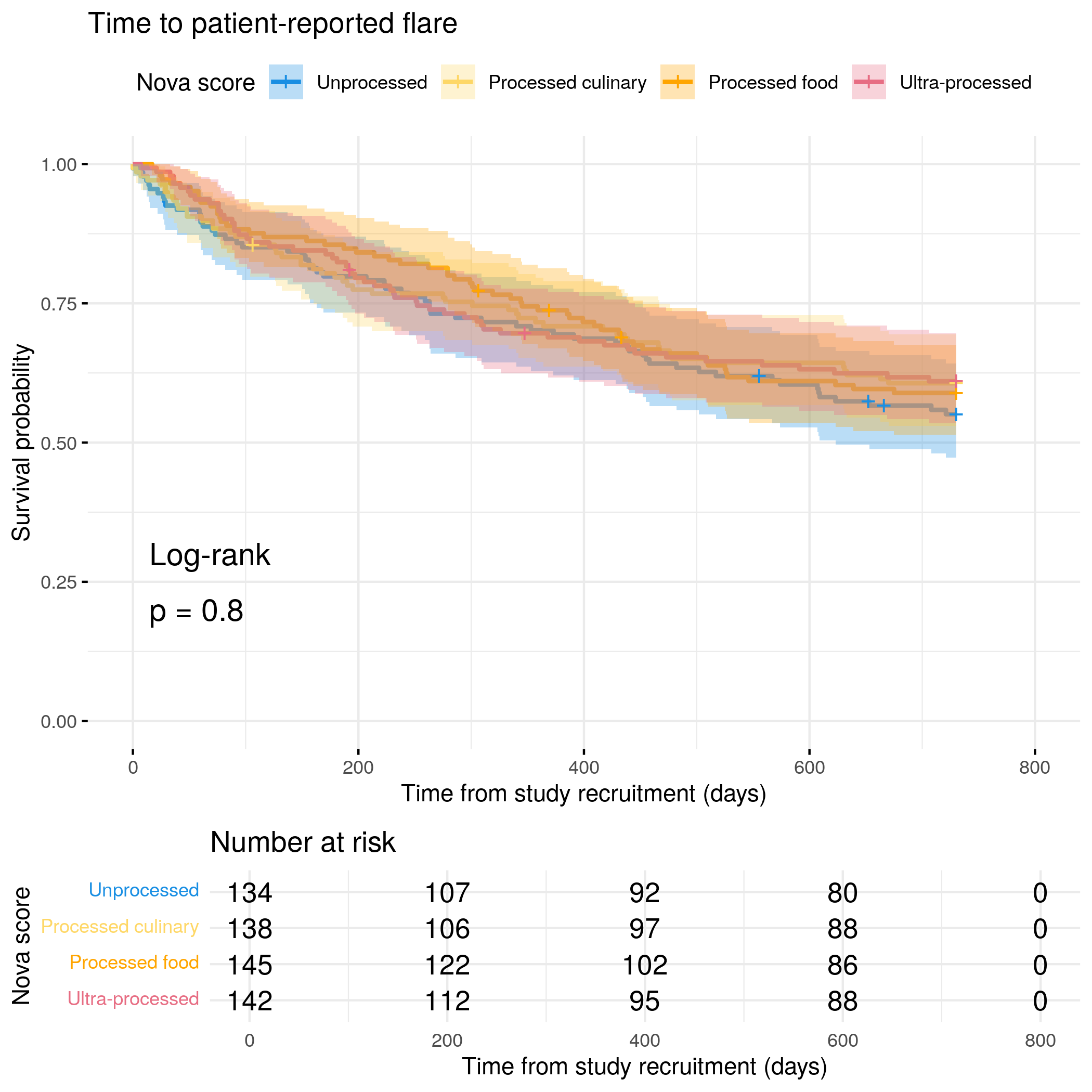
# Run survival analysis using utility functionanalysis_result<-run_survival_analysis( data =flare.df, var_name ="NOVAScore", outcome_time ="softflare_time", outcome_event ="softflare", legend_title ="Nova score", plot_base_path ="plots/ibd/soft-flare/diet/nova", break_time_by =200)# Run Cox model with categorical variablefit.me<-coxph(Surv(softflare_time, softflare)~Sex+cat+IMD+dqi_tot+BMI+NOVAScore_cat+frailty(SiteNo), control =coxph.control(outer.max =20), data =flare.df)hrs<-rbind(hrs, broom::tidy(fit.me)|>filter(!grepl("^Sex|^cat|^IMD|^dqi_tot|^BMI|^frailty", term))|>mutate(diagnosis ="IBD", flare ="Soft")|>relocate(diagnosis, flare))# Display plot and model summaryknitr::include_graphics("plots/ibd/soft-flare/diet/nova.png")
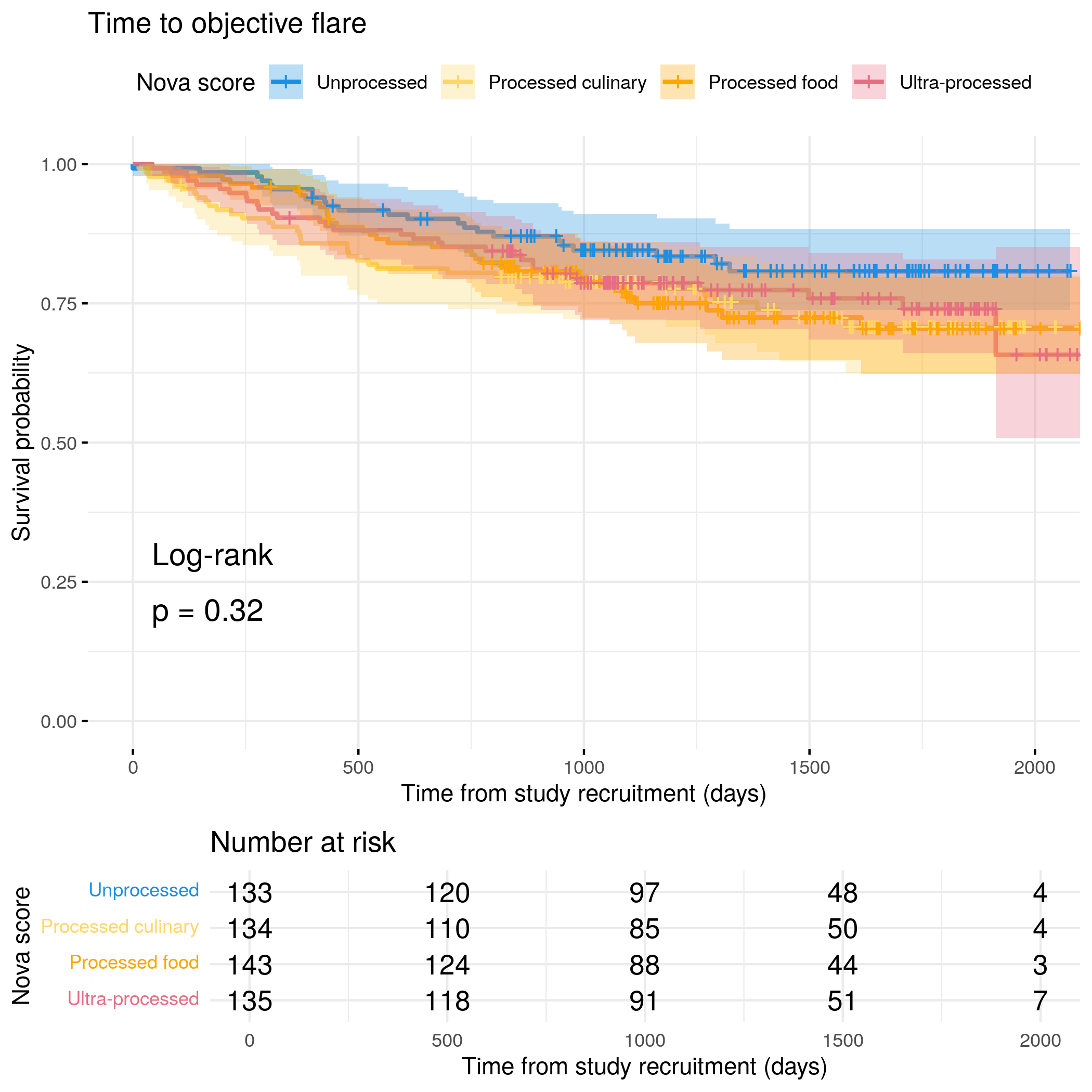
# Run survival analysis using utility function for objective flareanalysis_result<-run_survival_analysis( data =flare.df, var_name ="NOVAScore", outcome_time ="hardflare_time", outcome_event ="hardflare", legend_title ="Nova score", plot_base_path ="plots/ibd/hard-flare/diet/nova", break_time_by =500)# Run Cox model with categorical variablefit.me<-coxph(Surv(hardflare_time, hardflare)~Sex+cat+IMD+dqi_tot+BMI+NOVAScore_cat+frailty(SiteNo), control =coxph.control(outer.max =20), data =flare.df)hrs<-rbind(hrs, broom::tidy(fit.me)|>filter(!grepl("^Sex|^cat|^IMD|^dqi_tot|^BMI|^frailty", term))|>mutate(diagnosis ="IBD", flare ="Hard")|>relocate(diagnosis, flare))# Display plot and model summaryknitr::include_graphics("plots/ibd/hard-flare/diet/nova.png")
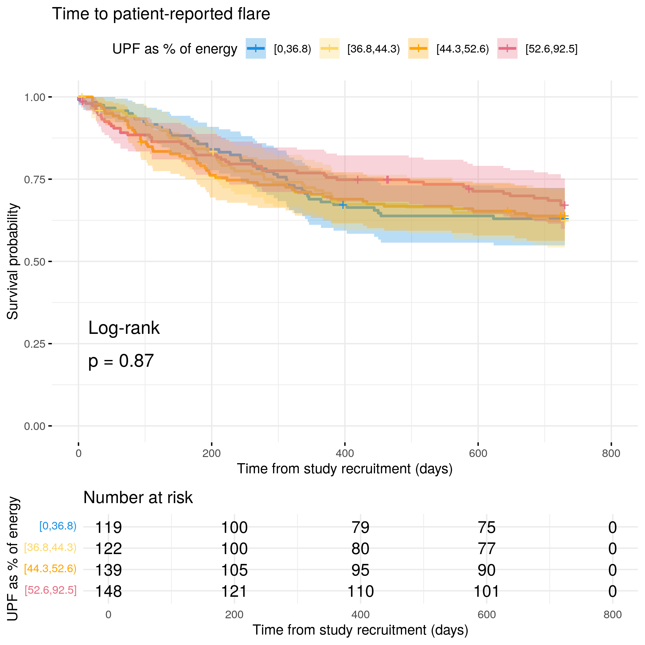
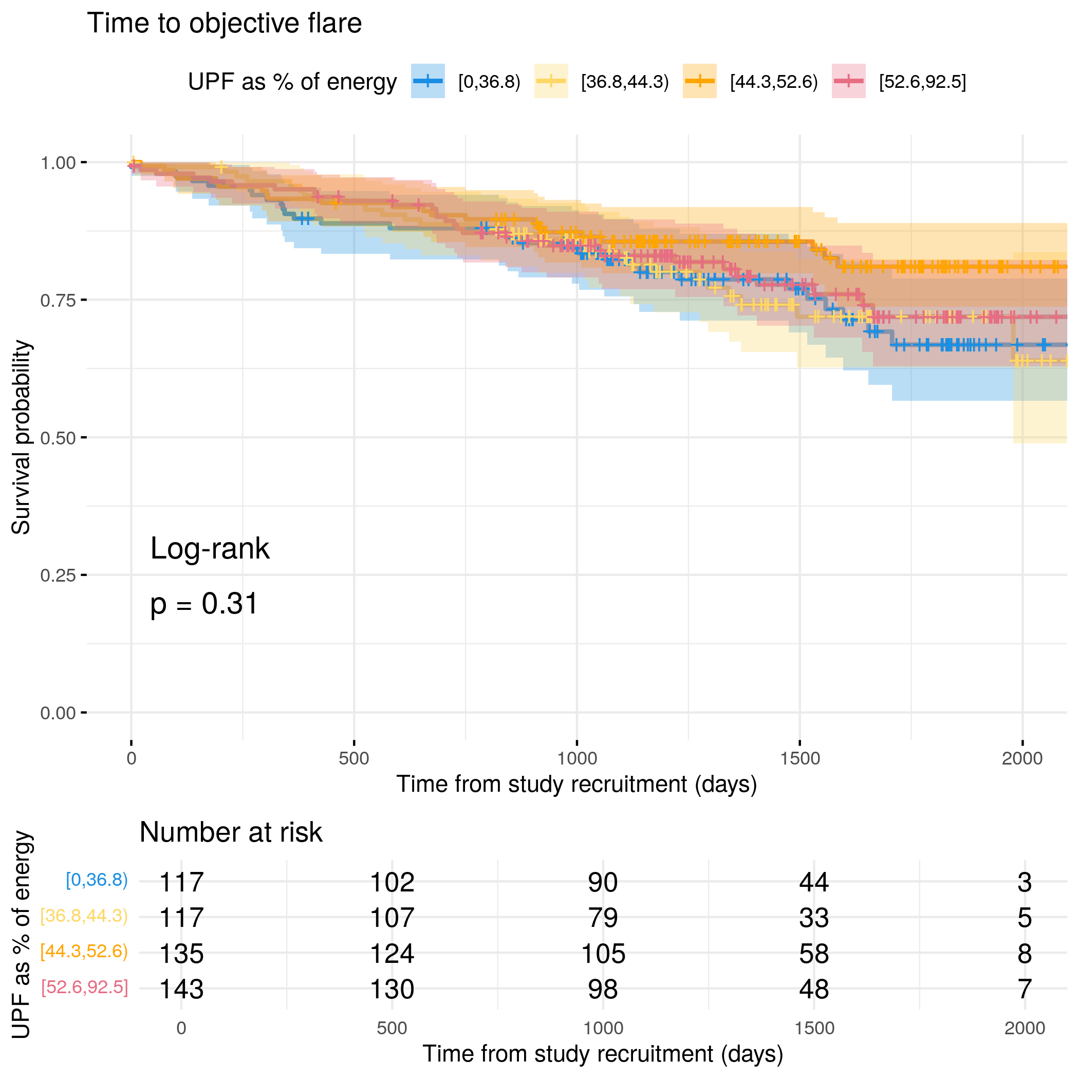
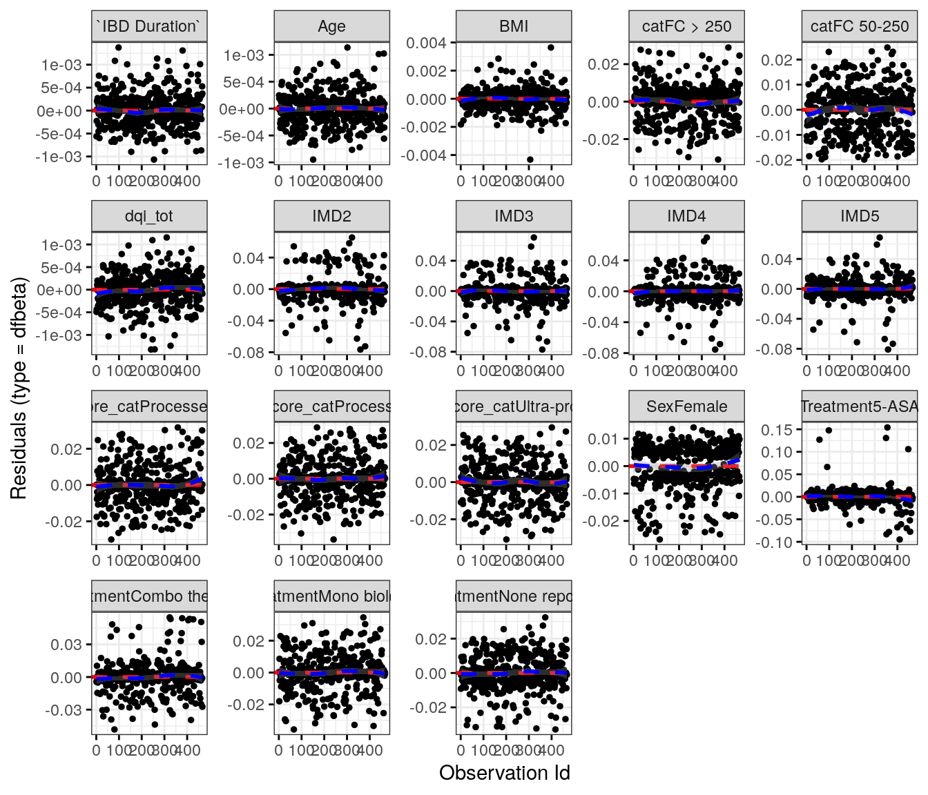
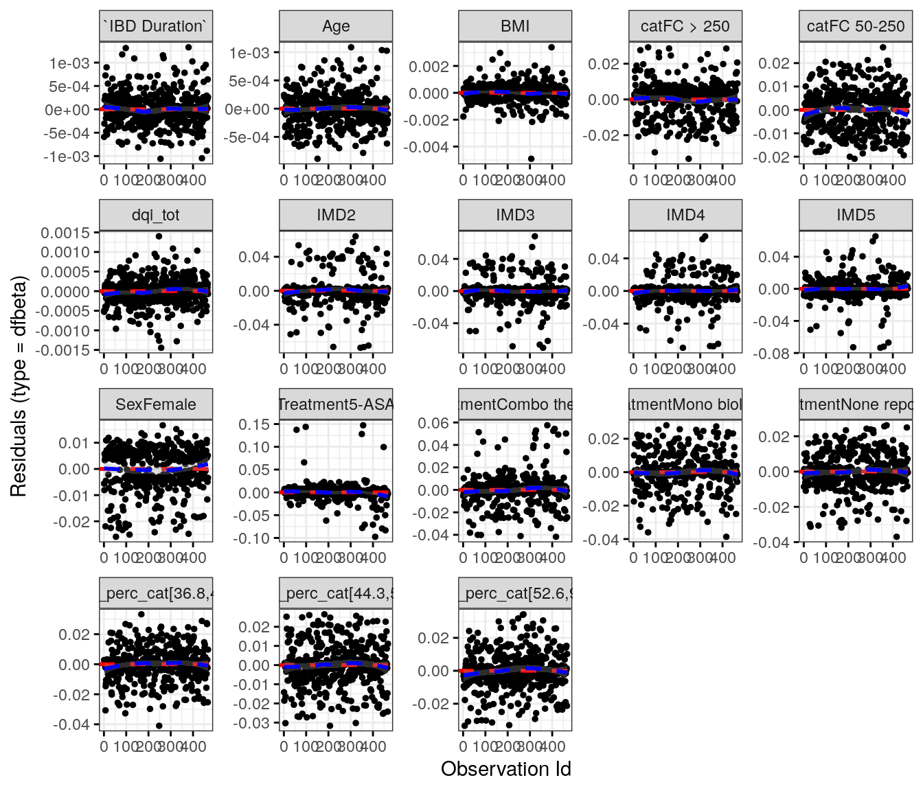
As an alternative approach to characterising ultra-processed food, we considered the percentage of daily energy intake sourced from ultra-processed food and drink (Nova 4).
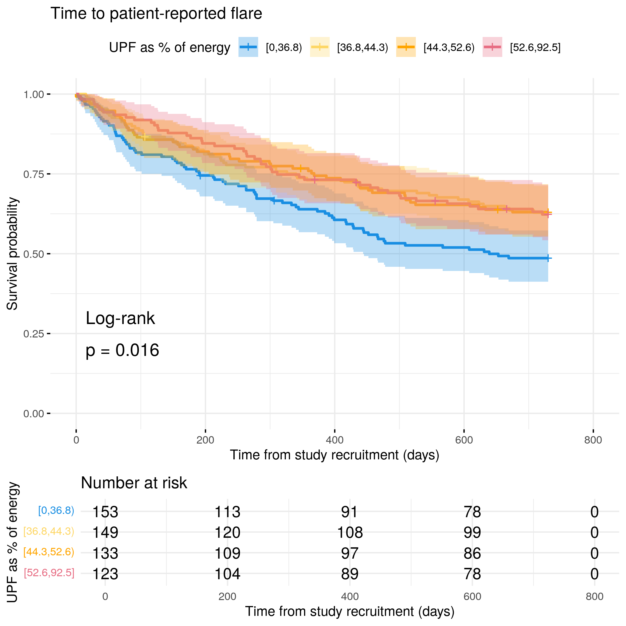
# Categorize UPF percentage by quantilesflare.cd.df<-categorize_by_quantiles(flare.cd.df, "UPF_perc", reference_data =flare.df)# Run survival analysis using utility functionanalysis_result<-run_survival_analysis( data =flare.cd.df, var_name ="UPF_perc", outcome_time ="softflare_time", outcome_event ="softflare", legend_title ="UPF as % of energy", plot_base_path ="plots/cd/soft-flare/diet/UPF", break_time_by =200)# Save plot as RDSsaveRDS(analysis_result$plot, paste0(paths$outdir, "upf-cd-soft.RDS"))# Run Cox model with categorical variablefit.me<-coxph(Surv(softflare_time, softflare)~Sex+cat+IMD+dqi_tot+BMI+UPF_perc_cat+frailty(SiteNo), control =coxph.control(outer.max =20), data =flare.cd.df)hrs<-rbind(hrs, broom::tidy(fit.me)|>filter(!grepl("^Sex|^cat|^IMD|^dqi_tot|^BMI|^frailty", term))|>mutate(diagnosis ="CD", flare ="Soft")|>relocate(diagnosis, flare))# Display plot and model summaryknitr::include_graphics("plots/cd/soft-flare/diet/UPF.png")
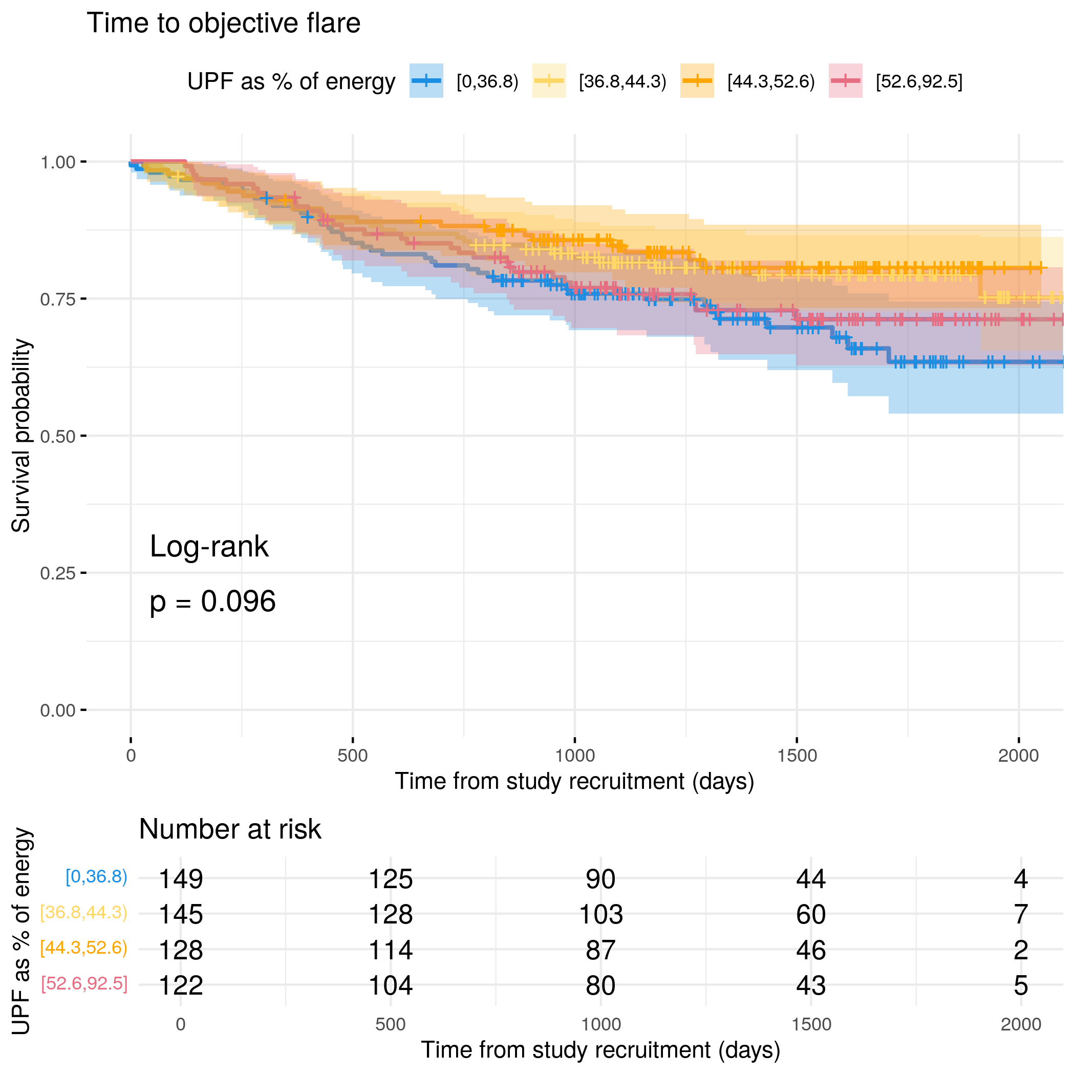
# Run survival analysis using utility function for objective flareanalysis_result<-run_survival_analysis( data =flare.cd.df, var_name ="UPF_perc", outcome_time ="hardflare_time", outcome_event ="hardflare", legend_title ="UPF as % of energy", plot_base_path ="plots/cd/hard-flare/diet/UPF", break_time_by =500)# Save plot as RDSsaveRDS(analysis_result$plot, paste0(paths$outdir, "upf-cd-hard.RDS"))# Run Cox model with categorical variablefit.me<-coxph(Surv(hardflare_time, hardflare)~Sex+cat+IMD+dqi_tot+BMI+UPF_perc_cat+frailty(SiteNo), control =coxph.control(outer.max =20), data =flare.cd.df)hrs<-rbind(hrs, broom::tidy(fit.me)|>filter(!grepl("^Sex|^cat|^IMD|^dqi_tot|^BMI|^frailty", term))|>mutate(diagnosis ="CD", flare ="Hard")|>relocate(diagnosis, flare))# Display plot and model summaryknitr::include_graphics("plots/cd/hard-flare/diet/UPF.png")
# Categorize UPF percentage by quantilesflare.uc.df<-categorize_by_quantiles(flare.uc.df, "UPF_perc", reference_data =flare.df)# Run survival analysis using utility functionanalysis_result<-run_survival_analysis( data =flare.uc.df, var_name ="UPF_perc", outcome_time ="softflare_time", outcome_event ="softflare", legend_title ="UPF as % of energy", plot_base_path ="plots/uc/soft-flare/diet/UPF", break_time_by =200)# Save plot as RDSsaveRDS(analysis_result$plot, paste0(paths$outdir, "upf-uc-soft.RDS"))# Run Cox model with categorical variablefit.me<-coxph(Surv(softflare_time, softflare)~Sex+cat+IMD+dqi_tot+BMI+UPF_perc_cat+frailty(SiteNo), control =coxph.control(outer.max =20), data =flare.uc.df)hrs<-rbind(hrs, broom::tidy(fit.me)|>filter(!grepl("^Sex|^cat|^IMD|^dqi_tot|^BMI|^frailty", term))|>mutate(diagnosis ="UC", flare ="Soft")|>relocate(diagnosis, flare))# Display plot and model summaryknitr::include_graphics("plots/uc/soft-flare/diet/UPF.png")
# Run survival analysis using utility function for objective flareanalysis_result<-run_survival_analysis( data =flare.uc.df, var_name ="UPF_perc", outcome_time ="hardflare_time", outcome_event ="hardflare", legend_title ="UPF as % of energy", plot_base_path ="plots/uc/hard-flare/diet/UPF", break_time_by =500)# Save plot as RDSsaveRDS(analysis_result$plot, paste0(paths$outdir, "upf-uc-hard.RDS"))# Run Cox model with categorical variablefit.me<-coxph(Surv(hardflare_time, hardflare)~Sex+cat+IMD+dqi_tot+BMI+UPF_perc_cat+frailty(SiteNo), control =coxph.control(outer.max =20), data =flare.uc.df)hrs<-rbind(hrs, broom::tidy(fit.me)|>filter(!grepl("^Sex|^cat|^IMD|^dqi_tot|^BMI|^frailty", term))|>mutate(diagnosis ="UC", flare ="Hard")|>relocate(diagnosis, flare))# Display plot and model summaryknitr::include_graphics("plots/uc/hard-flare/diet/UPF.png")
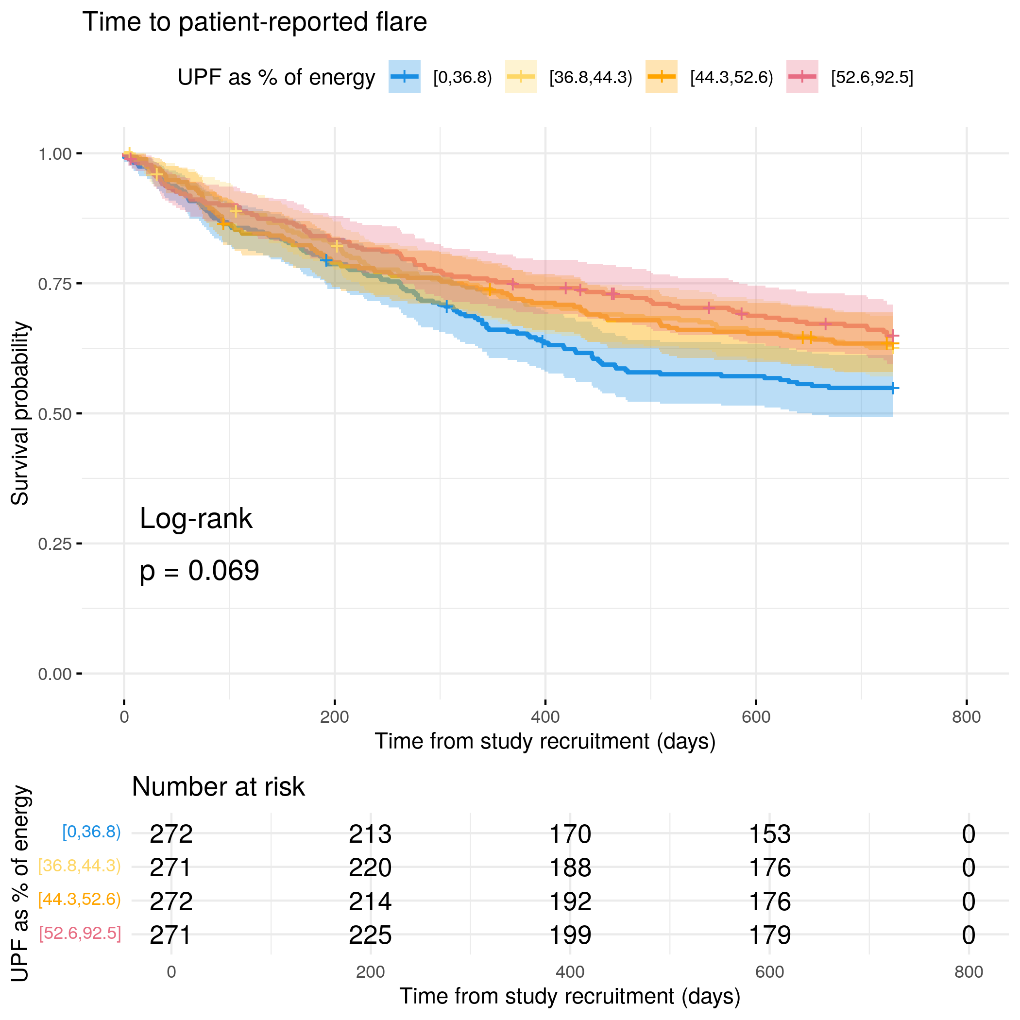
# Categorize UPF percentage by quantilesflare.df<-categorize_by_quantiles(flare.df, "UPF_perc", reference_data =flare.df)# Run survival analysis using utility functionanalysis_result<-run_survival_analysis( data =flare.df, var_name ="UPF_perc", outcome_time ="softflare_time", outcome_event ="softflare", legend_title ="UPF as % of energy", plot_base_path ="plots/ibd/soft-flare/diet/UPF", break_time_by =200)# Run Cox model with categorical variablefit.me<-coxph(Surv(softflare_time, softflare)~Sex+cat+IMD+dqi_tot+BMI+UPF_perc_cat+frailty(SiteNo), control =coxph.control(outer.max =20), data =flare.df)hrs<-rbind(hrs, broom::tidy(fit.me)|>filter(!grepl("^Sex|^cat|^IMD|^dqi_tot|^BMI|^frailty", term))|>mutate(diagnosis ="IBD", flare ="Soft")|>relocate(diagnosis, flare))# Display plot and model summaryknitr::include_graphics("plots/ibd/soft-flare/diet/UPF.png")
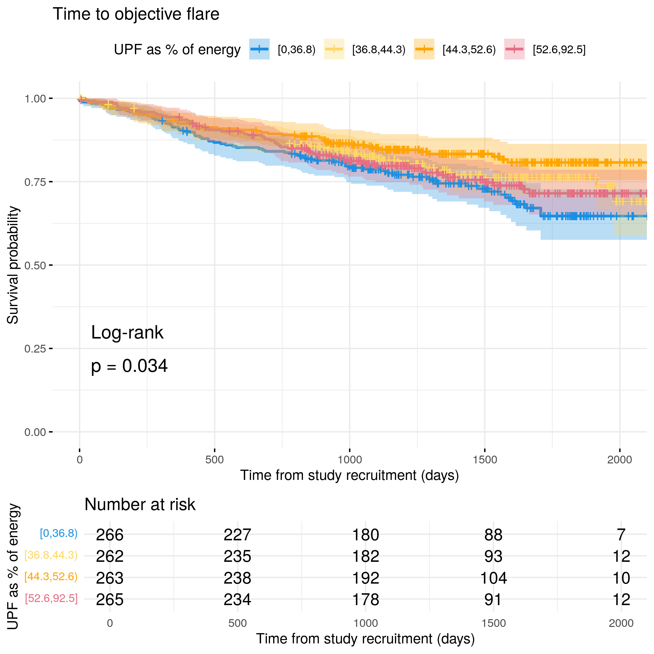
# Run survival analysis using utility function for objective flareanalysis_result<-run_survival_analysis( data =flare.df, var_name ="UPF_perc", outcome_time ="hardflare_time", outcome_event ="hardflare", legend_title ="UPF as % of energy", plot_base_path ="plots/ibd/hard-flare/diet/UPF", break_time_by =500)# Run Cox model with categorical variablefit.me<-coxph(Surv(hardflare_time, hardflare)~Sex+cat+IMD+dqi_tot+BMI+UPF_perc_cat+frailty(SiteNo), control =coxph.control(outer.max =20), data =flare.df)hrs<-rbind(hrs, broom::tidy(fit.me)|>filter(!grepl("^Sex|^cat|^IMD|^dqi_tot|^BMI|^frailty", term))|>mutate(diagnosis ="IBD", flare ="Hard")|>relocate(diagnosis, flare))# Display plot and model summaryknitr::include_graphics("plots/ibd/hard-flare/diet/UPF.png")
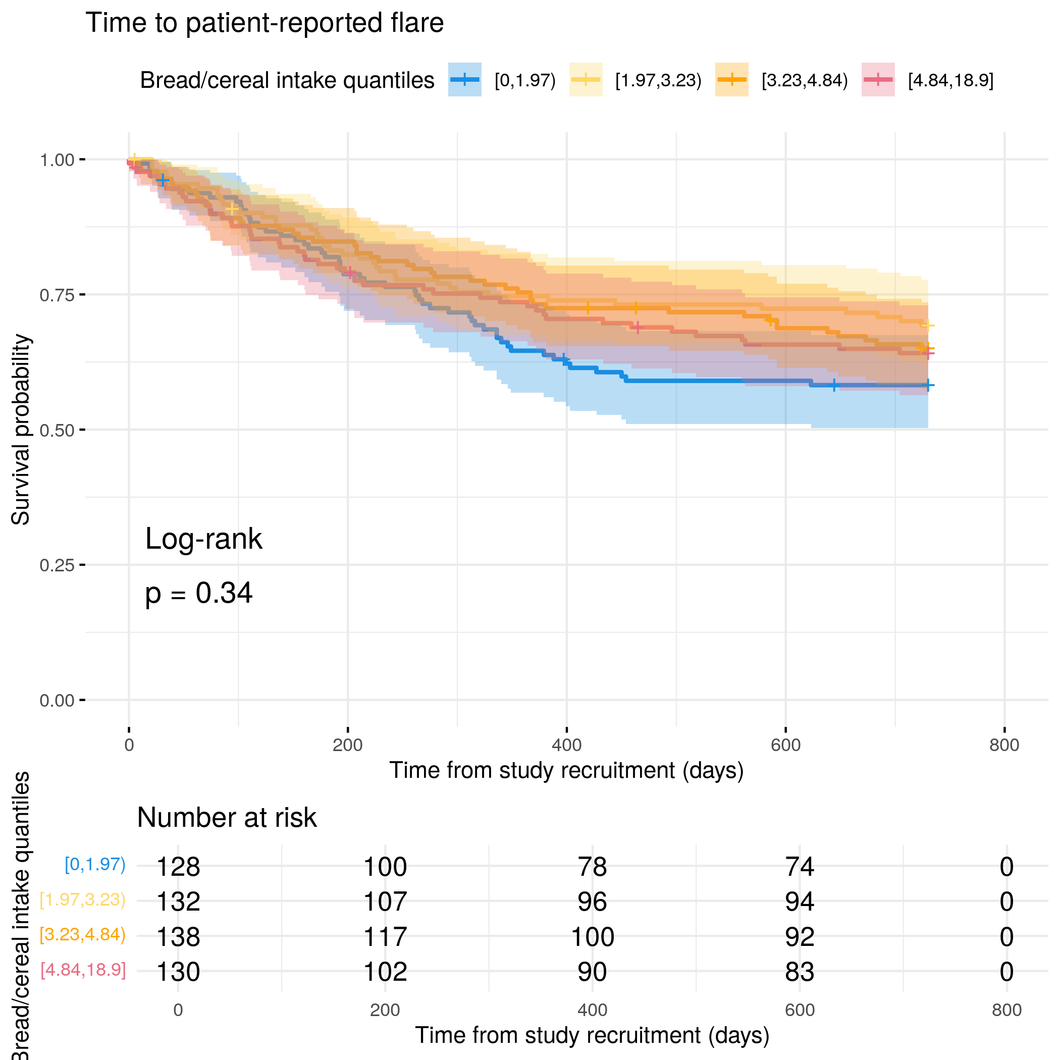
# Categorize bread intake by quantilesflare.cd.df<-categorize_by_quantiles(flare.cd.df, "breadIntake", reference_data =flare.df)# Run survival analysis using utility functionanalysis_result<-run_survival_analysis( data =flare.cd.df, var_name ="breadIntake", outcome_time ="softflare_time", outcome_event ="softflare", legend_title ="Bread/cereal intake quantiles", plot_base_path ="plots/cd/soft-flare/diet/breadIntake", break_time_by =200)# Save plot as RDSsaveRDS(analysis_result$plot, paste0(paths$outdir, "breadIntake-cd-soft.RDS"))# Run Cox model with categorical variablefit.me<-coxph(Surv(softflare_time, softflare)~Sex+cat+IMD+dqi_tot+BMI+breadIntake_cat+frailty(SiteNo), control =coxph.control(outer.max =20), data =flare.cd.df)hrs<-rbind(hrs, broom::tidy(fit.me)|>filter(!grepl("^Sex|^cat|^IMD|^dqi_tot|^BMI|^frailty", term))|>mutate(diagnosis ="CD", flare ="Soft")|>relocate(diagnosis, flare))# Display plot and model summaryknitr::include_graphics("plots/cd/soft-flare/diet/breadIntake.png")
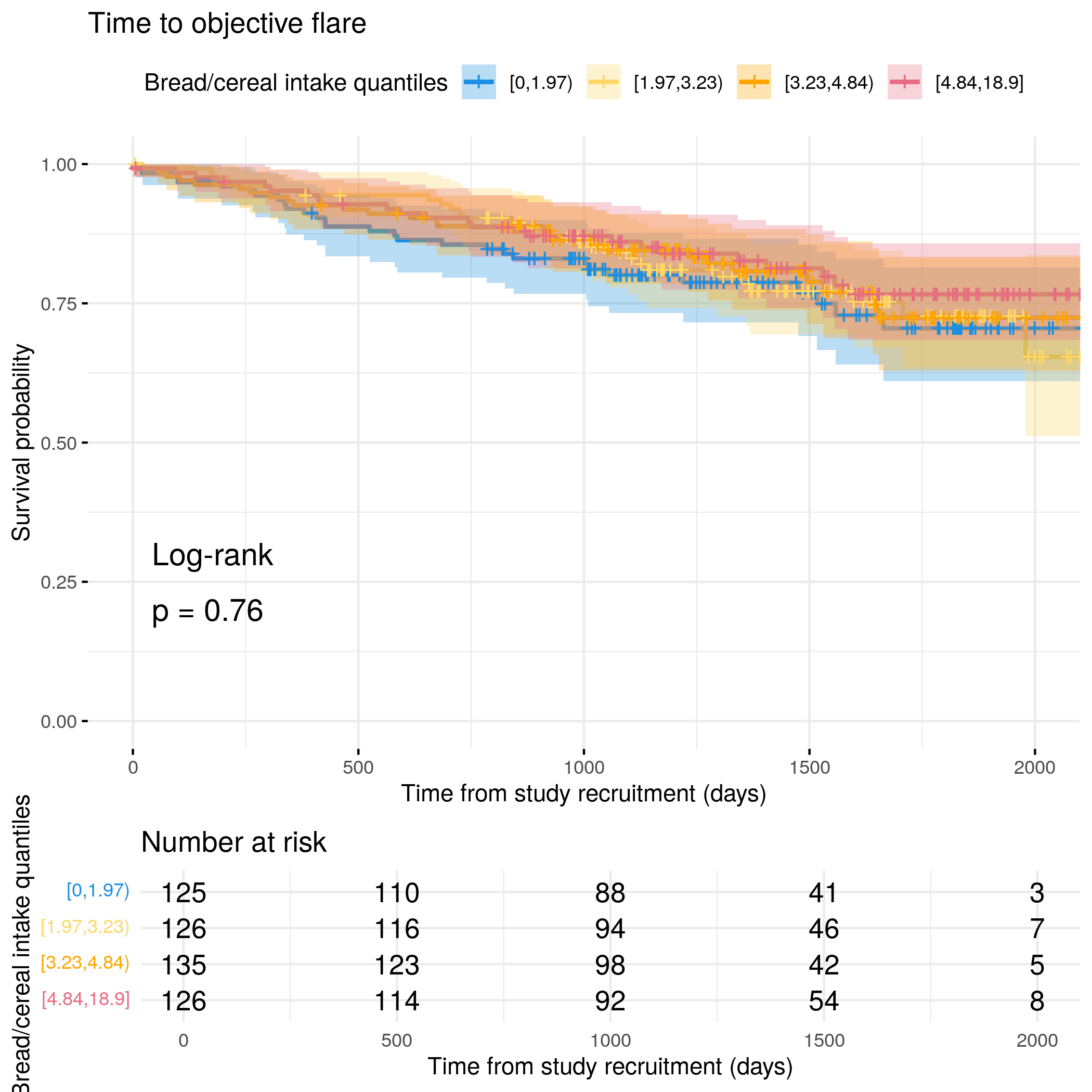
# Run survival analysis using utility function for objective flareanalysis_result<-run_survival_analysis( data =flare.cd.df, var_name ="breadIntake", outcome_time ="hardflare_time", outcome_event ="hardflare", legend_title ="Bread/cereal intake quantiles", plot_base_path ="plots/cd/hard-flare/diet/breadIntake", break_time_by =500)# Save plot as RDSsaveRDS(analysis_result$plot, paste0(paths$outdir, "breadIntake-cd-hard.RDS"))# Run Cox model with categorical variablefit.me<-coxph(Surv(hardflare_time, hardflare)~Sex+cat+IMD+dqi_tot+BMI+breadIntake_cat+frailty(SiteNo), control =coxph.control(outer.max =20), data =flare.cd.df)hrs<-rbind(hrs, broom::tidy(fit.me)|>filter(!grepl("^Sex|^cat|^IMD|^dqi_tot|^BMI|^frailty", term))|>mutate(diagnosis ="CD", flare ="Hard")|>relocate(diagnosis, flare))# Display plot and model summaryknitr::include_graphics("plots/cd/hard-flare/diet/breadIntake.png")
# Categorize bread intake by quantilesflare.uc.df<-categorize_by_quantiles(flare.uc.df, "breadIntake", reference_data =flare.df)# Run survival analysis using utility functionanalysis_result<-run_survival_analysis( data =flare.uc.df, var_name ="breadIntake", outcome_time ="softflare_time", outcome_event ="softflare", legend_title ="Bread/cereal intake quantiles", plot_base_path ="plots/uc/soft-flare/diet/breadIntake", break_time_by =200)# Save plot as RDSsaveRDS(analysis_result$plot, paste0(paths$outdir, "breadIntake-uc-soft.RDS"))# Run Cox model with categorical variablefit.me<-coxph(Surv(softflare_time, softflare)~Sex+cat+IMD+dqi_tot+BMI+breadIntake_cat+frailty(SiteNo), control =coxph.control(outer.max =20), data =flare.uc.df)hrs<-rbind(hrs, broom::tidy(fit.me)|>filter(!grepl("^Sex|^cat|^IMD|^dqi_tot|^BMI|^frailty", term))|>mutate(diagnosis ="UC", flare ="Soft")|>relocate(diagnosis, flare))# Display plot and model summaryknitr::include_graphics("plots/uc/soft-flare/diet/breadIntake.png")
# Run survival analysis using utility function for objective flareanalysis_result<-run_survival_analysis( data =flare.uc.df, var_name ="breadIntake", outcome_time ="hardflare_time", outcome_event ="hardflare", legend_title ="Bread/cereal intake quantiles", plot_base_path ="plots/uc/hard-flare/diet/breadIntake", break_time_by =500)# Save plot as RDSsaveRDS(analysis_result$plot, paste0(paths$outdir, "breadIntake-uc-hard.RDS"))# Run Cox model with categorical variablefit.me<-coxph(Surv(hardflare_time, hardflare)~Sex+cat+IMD+dqi_tot+BMI+breadIntake_cat+frailty(SiteNo), control =coxph.control(outer.max =20), data =flare.uc.df)hrs<-rbind(hrs, broom::tidy(fit.me)|>filter(!grepl("^Sex|^cat|^IMD|^dqi_tot|^BMI|^frailty", term))|>mutate(diagnosis ="UC", flare ="Hard")|>relocate(diagnosis, flare))# Display plot and model summaryknitr::include_graphics("plots/uc/hard-flare/diet/breadIntake.png")
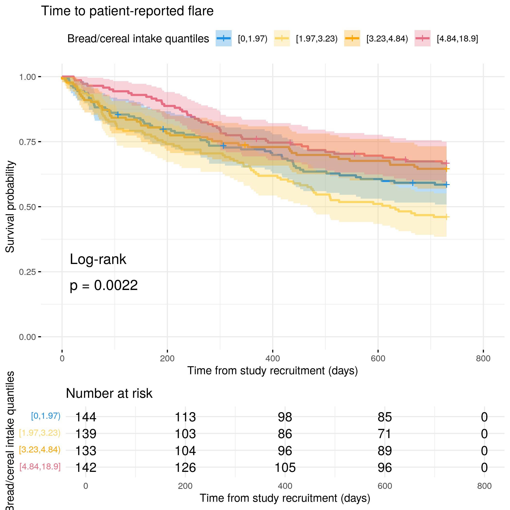
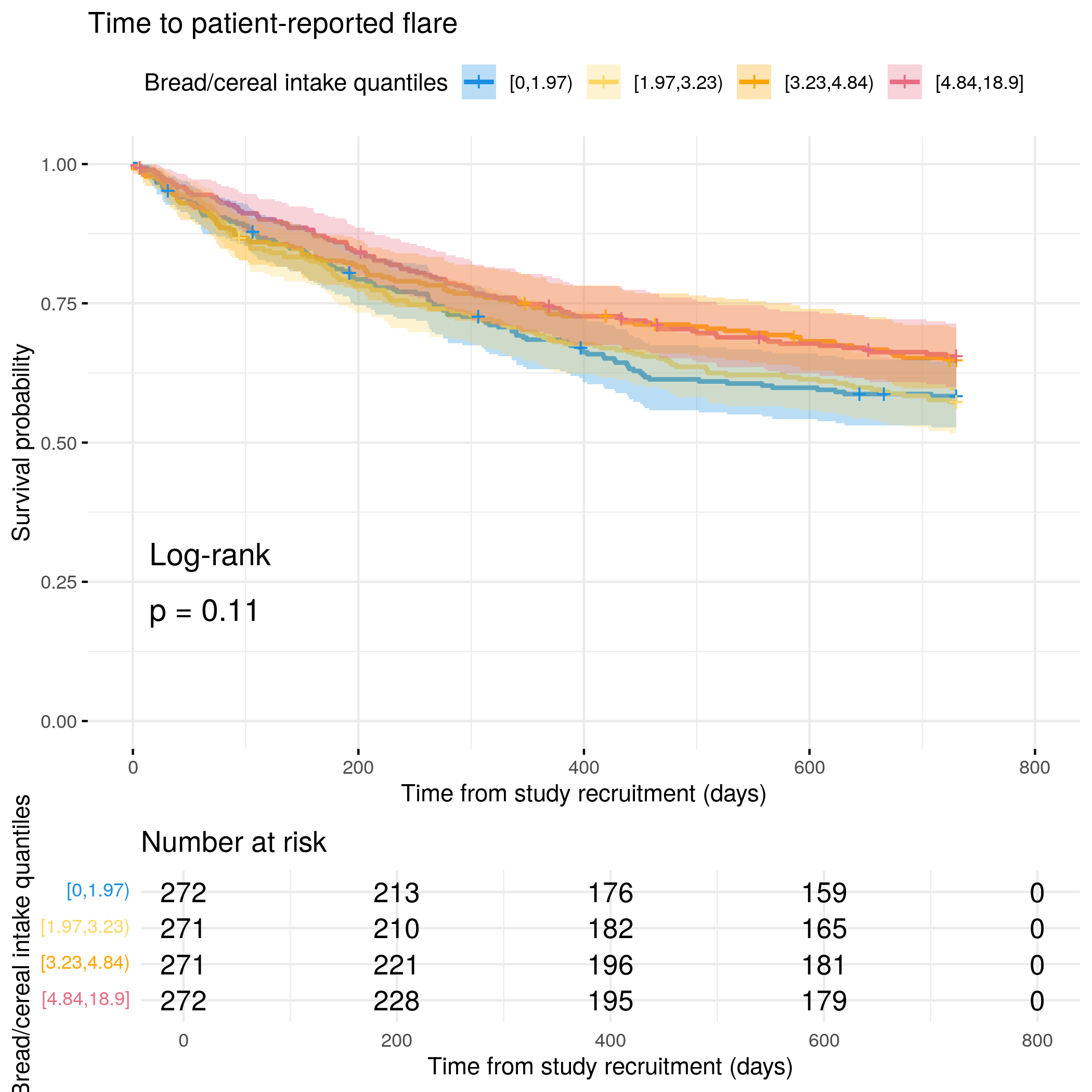
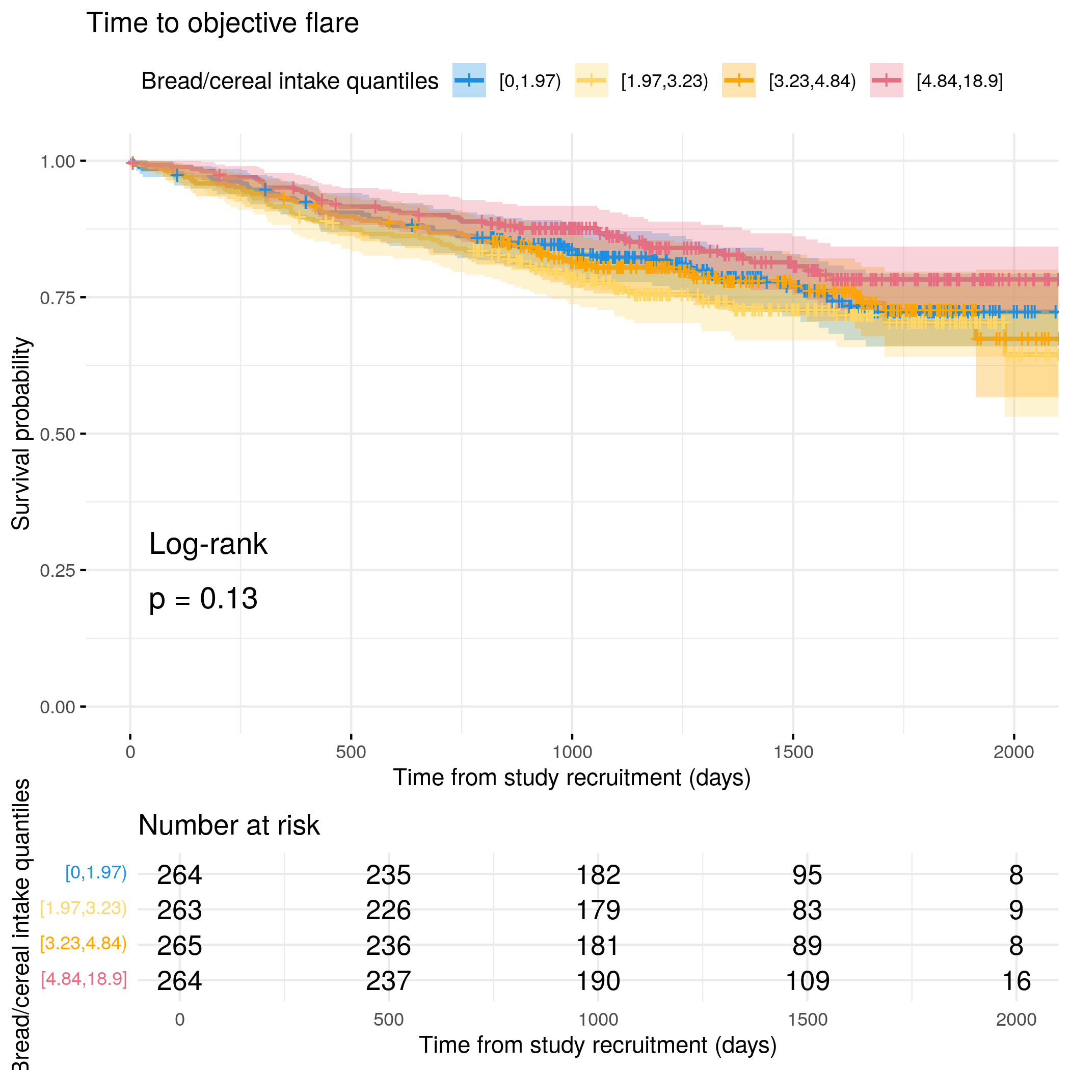
# Categorize bread intake by quantilesflare.df<-categorize_by_quantiles(flare.df, "breadIntake", reference_data =flare.df)# Run survival analysis using utility functionanalysis_result<-run_survival_analysis( data =flare.df, var_name ="breadIntake", outcome_time ="softflare_time", outcome_event ="softflare", legend_title ="Bread/cereal intake quantiles", plot_base_path ="plots/ibd/soft-flare/diet/breadIntake", break_time_by =200)# Run Cox model with categorical variablefit.me<-coxph(Surv(softflare_time, softflare)~Sex+cat+IMD+dqi_tot+BMI+breadIntake_cat+frailty(SiteNo), control =coxph.control(outer.max =20), data =flare.df)hrs<-rbind(hrs, broom::tidy(fit.me)|>filter(!grepl("^Sex|^cat|^IMD|^dqi_tot|^BMI|^frailty", term))|>mutate(diagnosis ="IBD", flare ="Soft")|>relocate(diagnosis, flare))# Display plot and model summaryknitr::include_graphics("plots/ibd/soft-flare/diet/breadIntake.png")
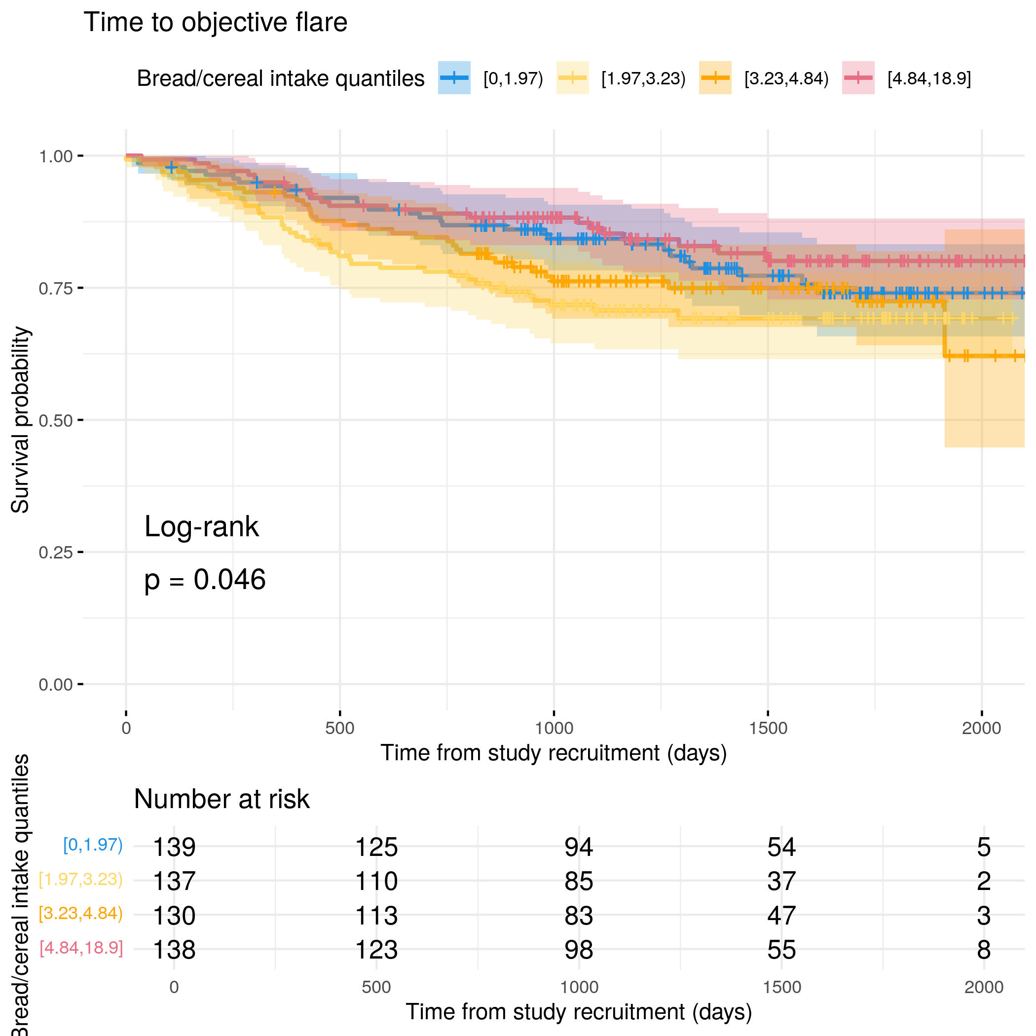
# Run survival analysis using utility function for objective flareanalysis_result<-run_survival_analysis( data =flare.df, var_name ="breadIntake", outcome_time ="hardflare_time", outcome_event ="hardflare", legend_title ="Bread/cereal intake quantiles", plot_base_path ="plots/ibd/hard-flare/diet/breadIntake", break_time_by =500)# Run Cox model with categorical variablefit.me<-coxph(Surv(hardflare_time, hardflare)~Sex+cat+IMD+dqi_tot+BMI+breadIntake_cat+frailty(SiteNo), control =coxph.control(outer.max =20), data =flare.df)hrs<-rbind(hrs, broom::tidy(fit.me)|>filter(!grepl("^Sex|^cat|^IMD|^dqi_tot|^BMI|^frailty", term))|>mutate(diagnosis ="IBD", flare ="Hard")|>relocate(diagnosis, flare))# Display plot and model summaryknitr::include_graphics("plots/ibd/hard-flare/diet/breadIntake.png")
# Categorize sweet intake by quantilesflare.cd.df<-categorize_by_quantiles(flare.cd.df, "sweetIntake", reference_data =flare.df)# Run survival analysis using utility functionanalysis_result<-run_survival_analysis( data =flare.cd.df, var_name ="sweetIntake", outcome_time ="softflare_time", outcome_event ="softflare", legend_title ="Sweet/dessert/snack intake quantiles", plot_base_path ="plots/cd/soft-flare/diet/sweetIntake", break_time_by =200)# Save plot as RDSsaveRDS(analysis_result$plot, paste0(paths$outdir, "sweetIntake-cd-soft.RDS"))# Run Cox model with categorical variablefit.me<-coxph(Surv(softflare_time, softflare)~Sex+cat+IMD+dqi_tot+BMI+sweetIntake_cat+frailty(SiteNo), control =coxph.control(outer.max =20), data =flare.cd.df)hrs<-rbind(hrs, broom::tidy(fit.me)|>filter(!grepl("^Sex|^cat|^IMD|^dqi_tot|^BMI|^frailty", term))|>mutate(diagnosis ="CD", flare ="Soft")|>relocate(diagnosis, flare))# Display plot and model summaryknitr::include_graphics("plots/cd/soft-flare/diet/sweetIntake.png")
# Run survival analysis using utility function for objective flareanalysis_result<-run_survival_analysis( data =flare.cd.df, var_name ="sweetIntake", outcome_time ="hardflare_time", outcome_event ="hardflare", legend_title ="Sweet/dessert/snack intake quantiles", plot_base_path ="plots/cd/hard-flare/diet/sweetIntake", break_time_by =500)# Save plot as RDSsaveRDS(analysis_result$plot, paste0(paths$outdir, "sweetIntake-cd-hard.RDS"))# Run Cox model with categorical variablefit.me<-coxph(Surv(hardflare_time, hardflare)~Sex+cat+IMD+dqi_tot+BMI+sweetIntake_cat+frailty(SiteNo), control =coxph.control(outer.max =20), data =flare.cd.df)hrs<-rbind(hrs, broom::tidy(fit.me)|>filter(!grepl("^Sex|^cat|^IMD|^dqi_tot|^BMI|^frailty", term))|>mutate(diagnosis ="CD", flare ="Hard")|>relocate(diagnosis, flare))# Display plot and model summaryknitr::include_graphics("plots/cd/hard-flare/diet/sweetIntake.png")
# Categorize sweet intake by quantilesflare.uc.df<-categorize_by_quantiles(flare.uc.df, "sweetIntake", reference_data =flare.df)# Run survival analysis using utility functionanalysis_result<-run_survival_analysis( data =flare.uc.df, var_name ="sweetIntake", outcome_time ="softflare_time", outcome_event ="softflare", legend_title ="Sweet/dessert/snack intake quantiles", plot_base_path ="plots/uc/soft-flare/diet/sweetIntake", break_time_by =200)# Save plot as RDSsaveRDS(analysis_result$plot, paste0(paths$outdir, "sweetIntake-uc-soft.RDS"))# Run Cox model with categorical variablefit.me<-coxph(Surv(softflare_time, softflare)~Sex+cat+IMD+dqi_tot+BMI+sweetIntake_cat+frailty(SiteNo), control =coxph.control(outer.max =20), data =flare.uc.df)hrs<-rbind(hrs, broom::tidy(fit.me)|>filter(!grepl("^Sex|^cat|^IMD|^dqi_tot|^BMI|^frailty", term))|>mutate(diagnosis ="UC", flare ="Soft")|>relocate(diagnosis, flare))# Display plot and model summaryknitr::include_graphics("plots/uc/soft-flare/diet/sweetIntake.png")
# Run survival analysis using utility function for objective flareanalysis_result<-run_survival_analysis( data =flare.uc.df, var_name ="sweetIntake", outcome_time ="hardflare_time", outcome_event ="hardflare", legend_title ="Sweet/dessert/snack intake quantiles", plot_base_path ="plots/uc/hard-flare/diet/sweetIntake", break_time_by =500)# Save plot as RDSsaveRDS(analysis_result$plot, paste0(paths$outdir, "sweetIntake-uc-hard.RDS"))# Run Cox model with categorical variablefit.me<-coxph(Surv(hardflare_time, hardflare)~Sex+cat+IMD+dqi_tot+BMI+sweetIntake_cat+frailty(SiteNo), control =coxph.control(outer.max =20), data =flare.uc.df)hrs<-rbind(hrs, broom::tidy(fit.me)|>filter(!grepl("^Sex|^cat|^IMD|^dqi_tot|^BMI|^frailty", term))|>mutate(diagnosis ="UC", flare ="Hard")|>relocate(diagnosis, flare))# Display plot and model summaryknitr::include_graphics("plots/uc/hard-flare/diet/sweetIntake.png")
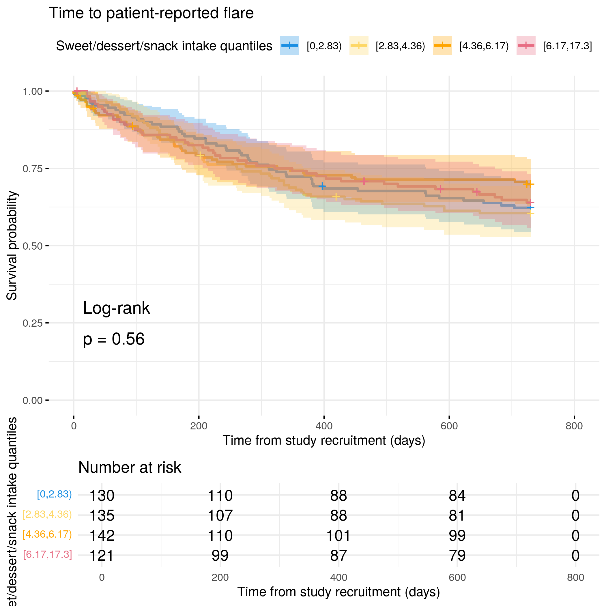
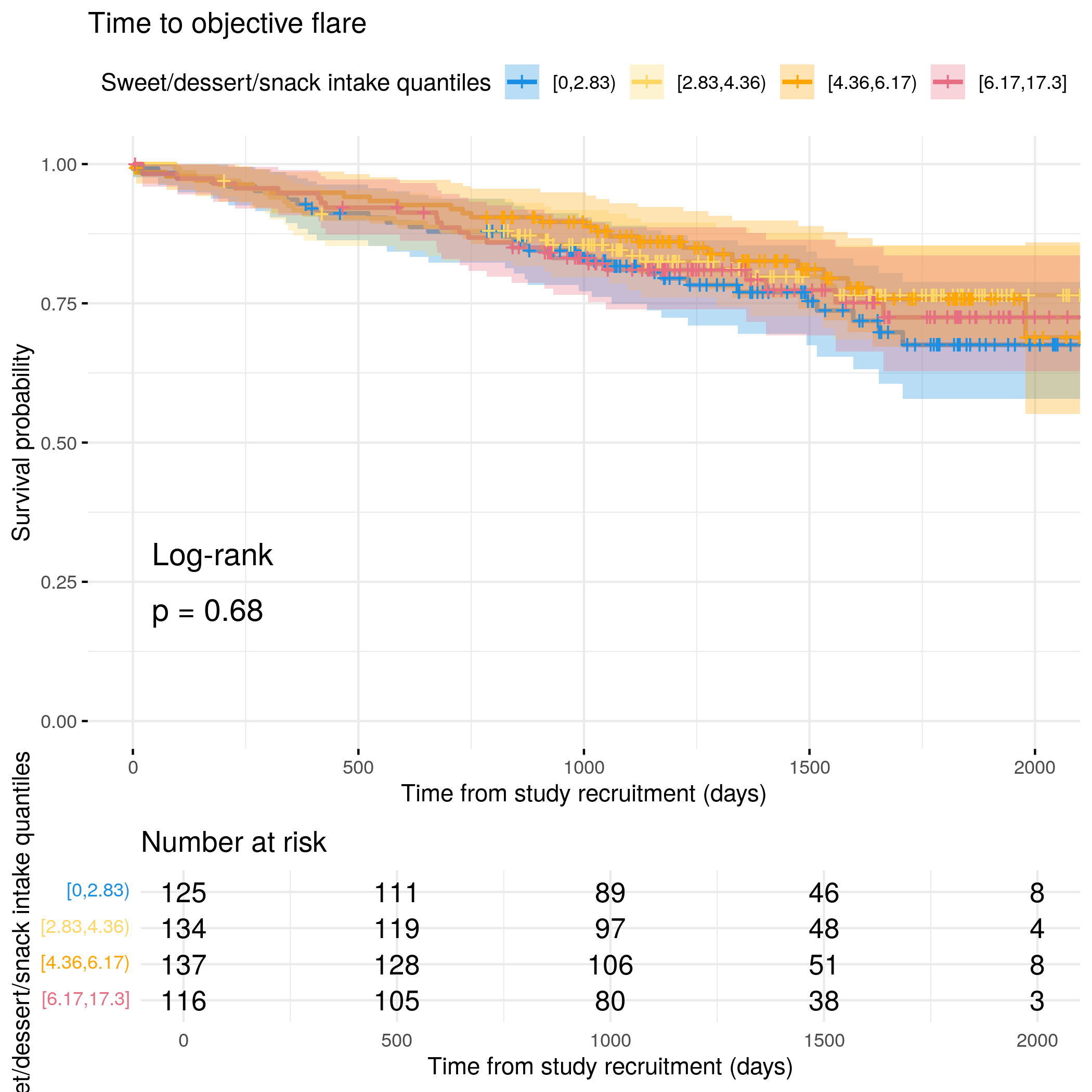
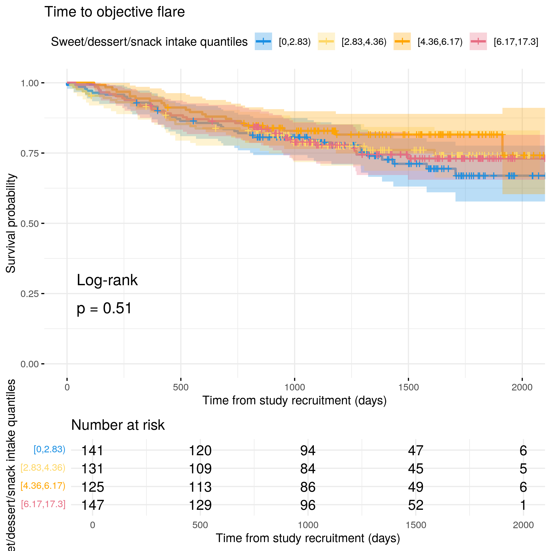
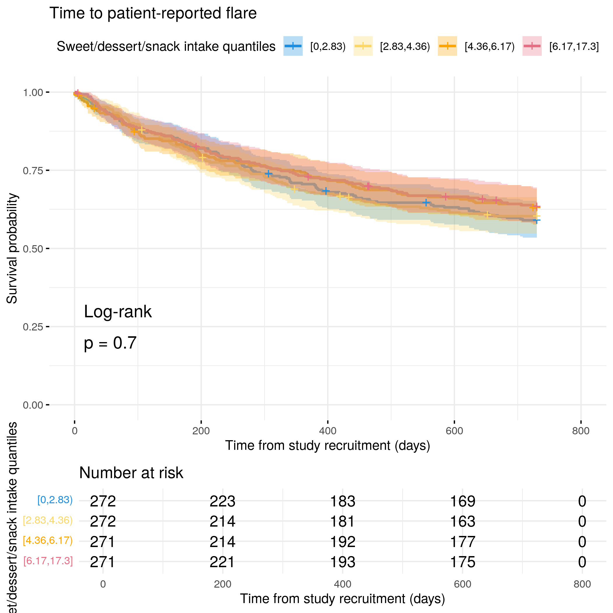
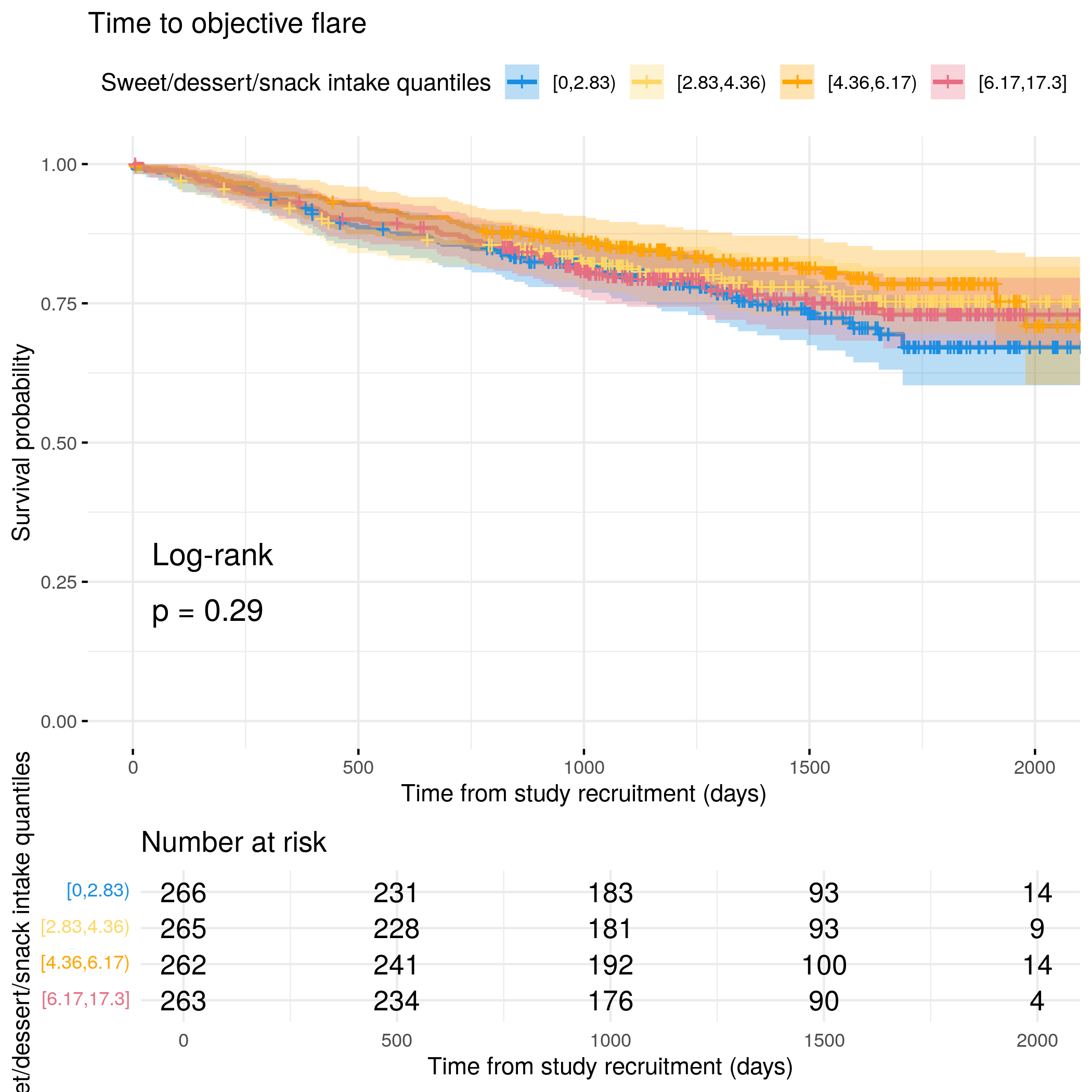
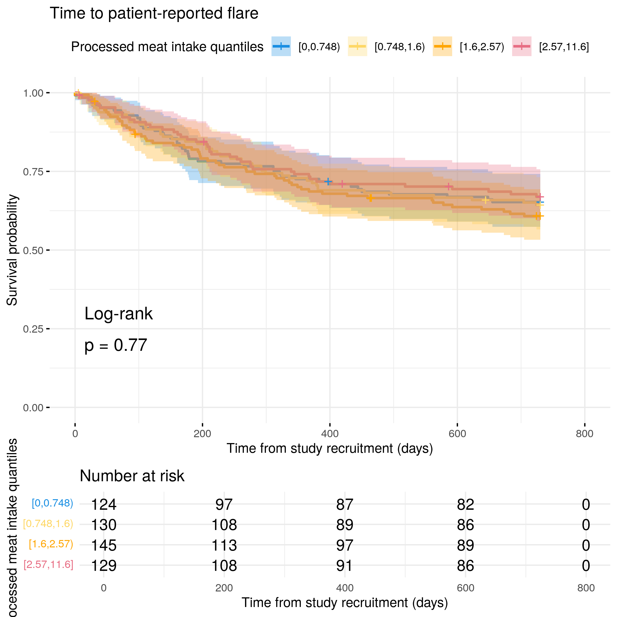
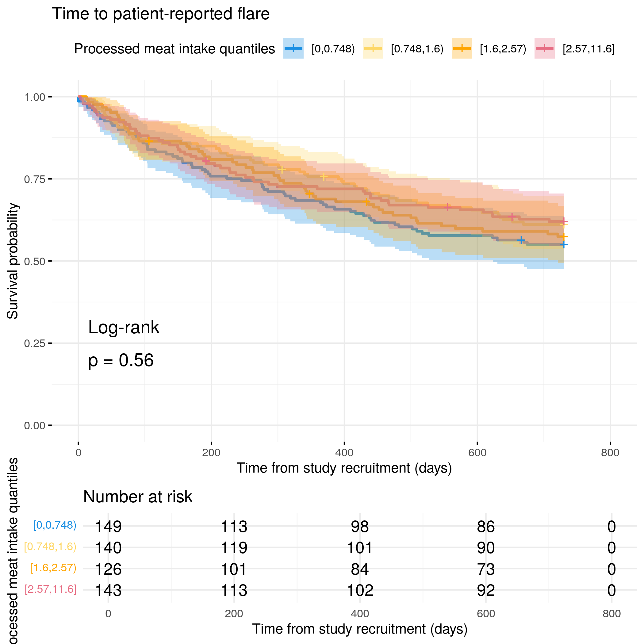
# Categorize sweet intake by quantilesflare.df<-categorize_by_quantiles(flare.df, "sweetIntake", reference_data =flare.df)# Run survival analysis using utility functionanalysis_result<-run_survival_analysis( data =flare.df, var_name ="sweetIntake", outcome_time ="softflare_time", outcome_event ="softflare", legend_title ="Sweet/dessert/snack intake quantiles", plot_base_path ="plots/ibd/soft-flare/diet/sweetIntake", break_time_by =200)# Run Cox model with categorical variablefit.me<-coxph(Surv(softflare_time, softflare)~Sex+cat+IMD+dqi_tot+BMI+sweetIntake_cat+frailty(SiteNo), control =coxph.control(outer.max =20), data =flare.df)hrs<-rbind(hrs, broom::tidy(fit.me)|>filter(!grepl("^Sex|^cat|^IMD|^dqi_tot|^BMI|^frailty", term))|>mutate(diagnosis ="IBD", flare ="Soft")|>relocate(diagnosis, flare))# Display plot and model summaryknitr::include_graphics("plots/ibd/soft-flare/diet/sweetIntake.png")
# Run survival analysis using utility function for objective flareanalysis_result<-run_survival_analysis( data =flare.df, var_name ="sweetIntake", outcome_time ="hardflare_time", outcome_event ="hardflare", legend_title ="Sweet/dessert/snack intake quantiles", plot_base_path ="plots/ibd/hard-flare/diet/sweetIntake", break_time_by =500)# Run Cox model with categorical variablefit.me<-coxph(Surv(hardflare_time, hardflare)~Sex+cat+IMD+dqi_tot+BMI+sweetIntake_cat+frailty(SiteNo), control =coxph.control(outer.max =20), data =flare.df)hrs<-rbind(hrs, broom::tidy(fit.me)|>filter(!grepl("^Sex|^cat|^IMD|^dqi_tot|^BMI|^frailty", term))|>mutate(diagnosis ="IBD", flare ="Hard")|>relocate(diagnosis, flare))# Display plot and model summaryknitr::include_graphics("plots/ibd/hard-flare/diet/sweetIntake.png")
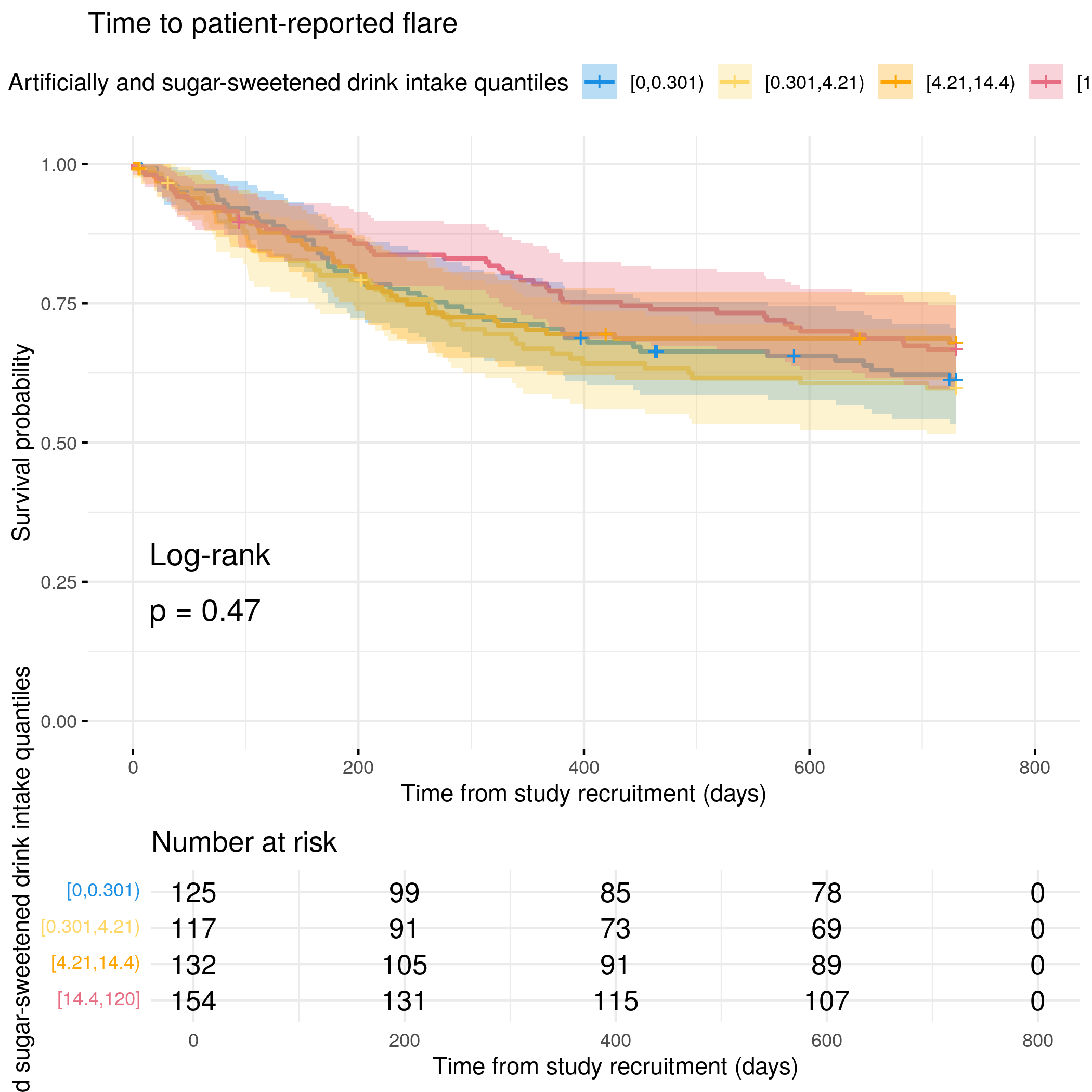
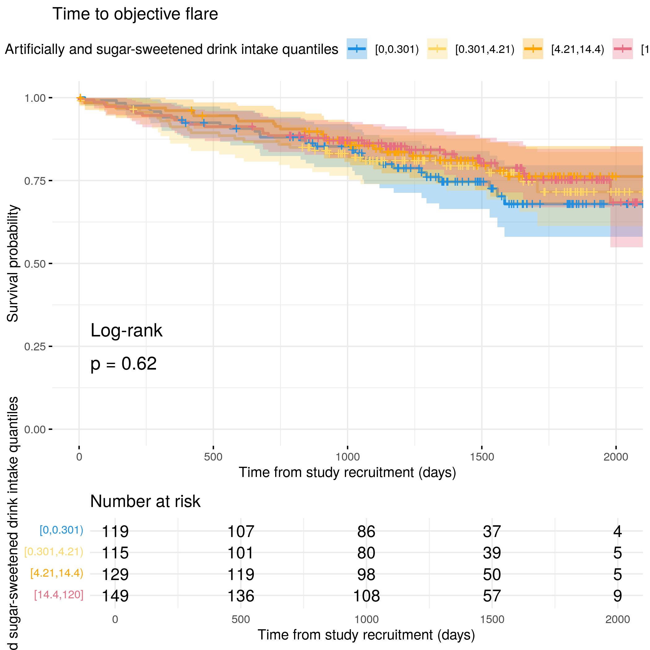
# Categorize drink intake by quantilesflare.cd.df<-categorize_by_quantiles(flare.cd.df, "drinkIntake", reference_data =flare.df)# Run survival analysis using utility functionanalysis_result<-run_survival_analysis( data =flare.cd.df, var_name ="drinkIntake", outcome_time ="softflare_time", outcome_event ="softflare", legend_title ="Artificially and sugar-sweetened drink intake quantiles", plot_base_path ="plots/cd/soft-flare/diet/drinkIntake", break_time_by =200)# Save plot as RDSsaveRDS(analysis_result$plot, paste0(paths$outdir, "drinkIntake-cd-soft.RDS"))# Run Cox model with categorical variablefit.me<-coxph(Surv(softflare_time, softflare)~Sex+cat+IMD+dqi_tot+BMI+drinkIntake_cat+frailty(SiteNo), control =coxph.control(outer.max =20), data =flare.cd.df)hrs<-rbind(hrs, broom::tidy(fit.me)|>filter(!grepl("^Sex|^cat|^IMD|^dqi_tot|^BMI|^frailty", term))|>mutate(diagnosis ="CD", flare ="Soft")|>relocate(diagnosis, flare))# Display plot and model summaryknitr::include_graphics("plots/cd/soft-flare/diet/drinkIntake.png")
# Run survival analysis using utility function for objective flareanalysis_result<-run_survival_analysis( data =flare.cd.df, var_name ="drinkIntake", outcome_time ="hardflare_time", outcome_event ="hardflare", legend_title ="Artificially and sugar-sweetened drink intake quantiles", plot_base_path ="plots/cd/hard-flare/diet/drinkIntake", break_time_by =500)# Save plot as RDSsaveRDS(analysis_result$plot, paste0(paths$outdir, "drinkIntake-cd-hard.RDS"))# Run Cox model with categorical variablefit.me<-coxph(Surv(hardflare_time, hardflare)~Sex+cat+IMD+dqi_tot+BMI+drinkIntake_cat+frailty(SiteNo), control =coxph.control(outer.max =20), data =flare.cd.df)hrs<-rbind(hrs, broom::tidy(fit.me)|>filter(!grepl("^Sex|^cat|^IMD|^dqi_tot|^BMI|^frailty", term))|>mutate(diagnosis ="CD", flare ="Hard")|>relocate(diagnosis, flare))# Display plot and model summaryknitr::include_graphics("plots/cd/hard-flare/diet/drinkIntake.png")
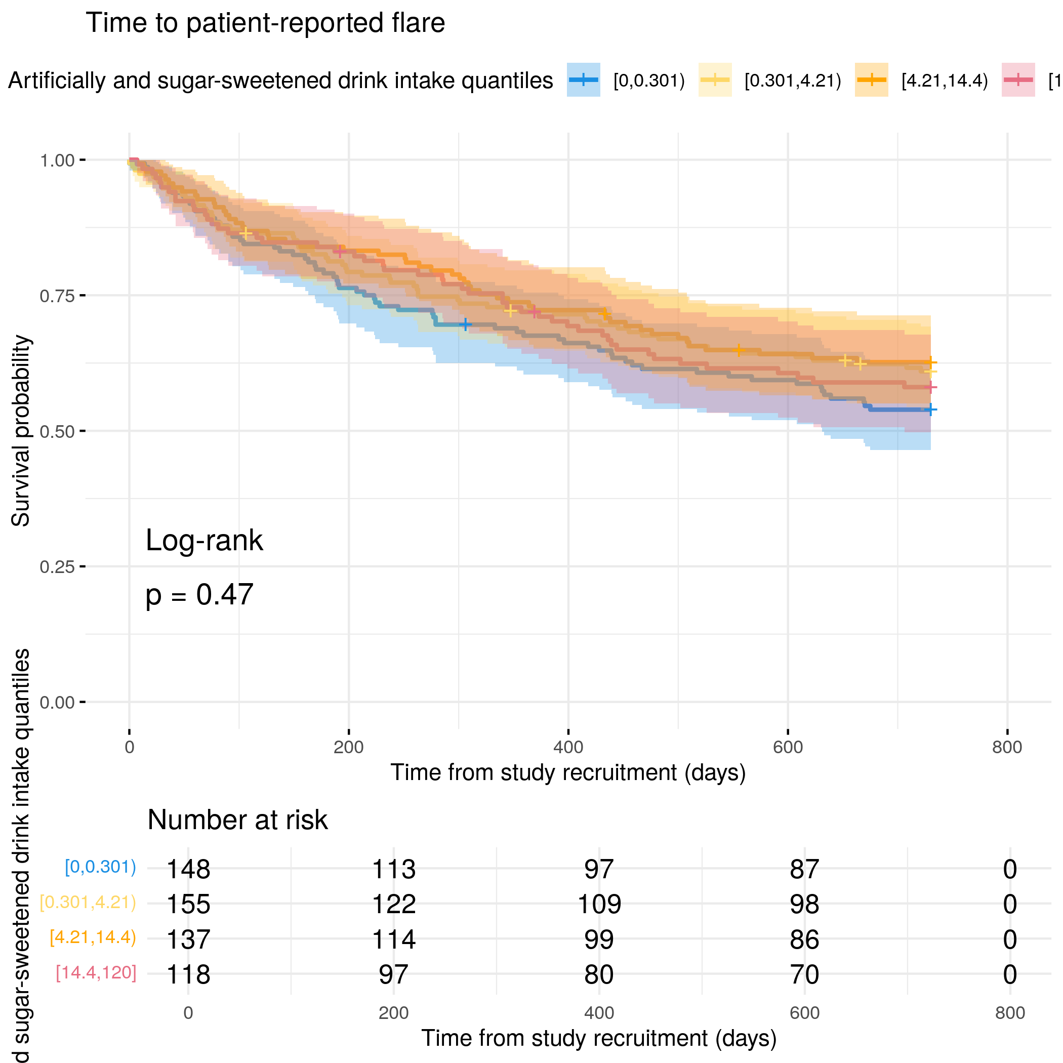
# Categorize drink intake by quantilesflare.uc.df<-categorize_by_quantiles(flare.uc.df, "drinkIntake", reference_data =flare.df)# Run survival analysis using utility functionanalysis_result<-run_survival_analysis( data =flare.uc.df, var_name ="drinkIntake", outcome_time ="softflare_time", outcome_event ="softflare", legend_title ="Artificially and sugar-sweetened drink intake quantiles", plot_base_path ="plots/uc/soft-flare/diet/drinkIntake", break_time_by =200)# Save plot as RDSsaveRDS(analysis_result$plot, paste0(paths$outdir, "drinkIntake-uc-soft.RDS"))# Run Cox model with categorical variablefit.me<-coxph(Surv(softflare_time, softflare)~Sex+cat+IMD+dqi_tot+BMI+drinkIntake_cat+frailty(SiteNo), control =coxph.control(outer.max =20), data =flare.uc.df)hrs<-rbind(hrs, broom::tidy(fit.me)|>filter(!grepl("^Sex|^cat|^IMD|^dqi_tot|^BMI|^frailty", term))|>mutate(diagnosis ="UC", flare ="Soft")|>relocate(diagnosis, flare))# Display plot and model summaryknitr::include_graphics("plots/uc/soft-flare/diet/drinkIntake.png")
# Run survival analysis using utility function for objective flareanalysis_result<-run_survival_analysis( data =flare.uc.df, var_name ="drinkIntake", outcome_time ="hardflare_time", outcome_event ="hardflare", legend_title ="Artificially and sugar-sweetened drink intake quantiles", plot_base_path ="plots/uc/hard-flare/diet/drinkIntake", break_time_by =500)# Save plot as RDSsaveRDS(analysis_result$plot, paste0(paths$outdir, "drinkIntake-uc-hard.RDS"))# Run Cox model with categorical variablefit.me<-coxph(Surv(hardflare_time, hardflare)~Sex+cat+IMD+dqi_tot+BMI+drinkIntake_cat+frailty(SiteNo), control =coxph.control(outer.max =20), data =flare.uc.df)hrs<-rbind(hrs, broom::tidy(fit.me)|>filter(!grepl("^Sex|^cat|^IMD|^dqi_tot|^BMI|^frailty", term))|>mutate(diagnosis ="UC", flare ="Hard")|>relocate(diagnosis, flare))# Display plot and model summaryknitr::include_graphics("plots/uc/hard-flare/diet/drinkIntake.png")
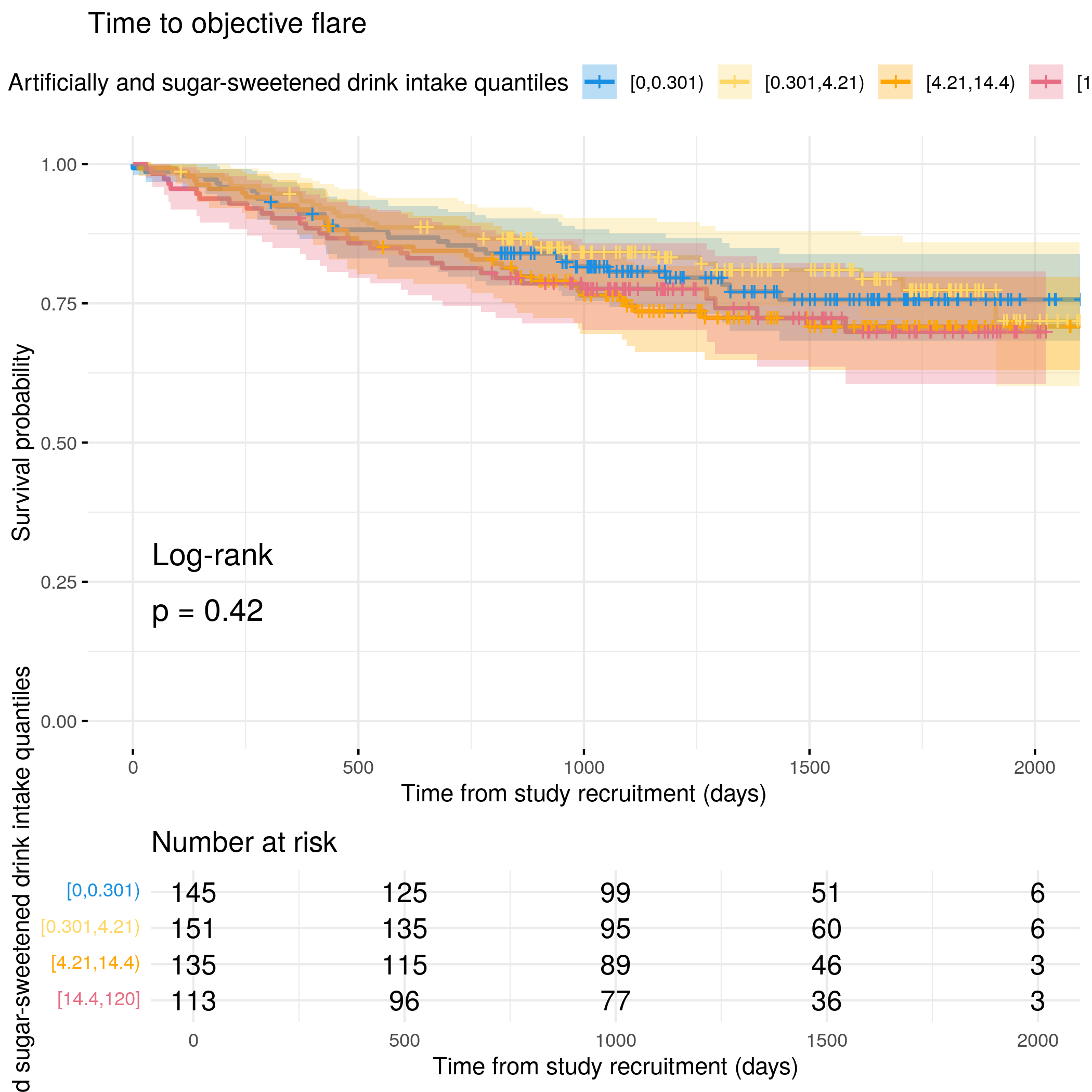
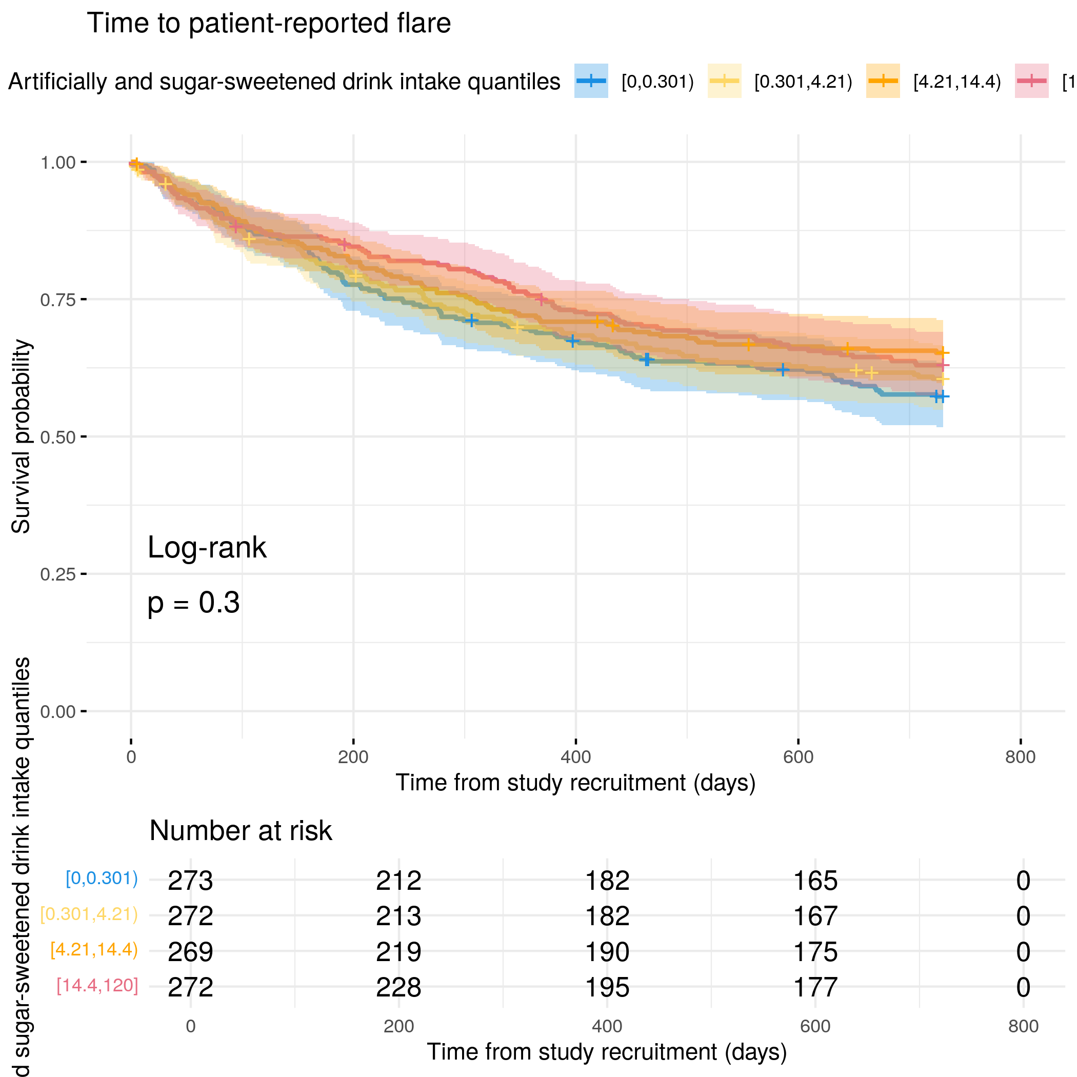
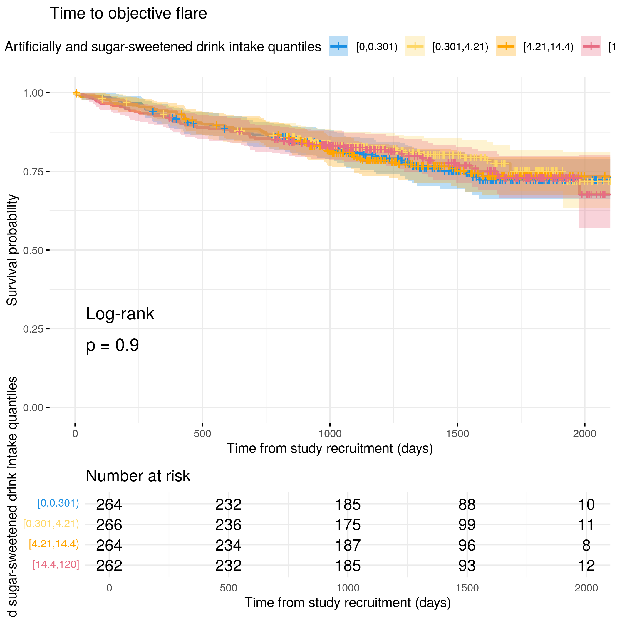
# Categorize drink intake by quantilesflare.df<-categorize_by_quantiles(flare.df, "drinkIntake", reference_data =flare.df)# Run survival analysis using utility functionanalysis_result<-run_survival_analysis( data =flare.df, var_name ="drinkIntake", outcome_time ="softflare_time", outcome_event ="softflare", legend_title ="Artificially and sugar-sweetened drink intake quantiles", plot_base_path ="plots/ibd/soft-flare/diet/drinkIntake", break_time_by =200)# Run Cox model with categorical variablefit.me<-coxph(Surv(softflare_time, softflare)~Sex+cat+IMD+dqi_tot+BMI+drinkIntake_cat+frailty(SiteNo), control =coxph.control(outer.max =20), data =flare.df)hrs<-rbind(hrs, broom::tidy(fit.me)|>filter(!grepl("^Sex|^cat|^IMD|^dqi_tot|^BMI|^frailty", term))|>mutate(diagnosis ="IBD", flare ="Soft")|>relocate(diagnosis, flare))# Display plot and model summaryknitr::include_graphics("plots/ibd/soft-flare/diet/drinkIntake.png")
# Run survival analysis using utility function for objective flareanalysis_result<-run_survival_analysis( data =flare.df, var_name ="drinkIntake", outcome_time ="hardflare_time", outcome_event ="hardflare", legend_title ="Artificially and sugar-sweetened drink intake quantiles", plot_base_path ="plots/ibd/hard-flare/diet/drinkIntake", break_time_by =500)# Run Cox model with categorical variablefit.me<-coxph(Surv(hardflare_time, hardflare)~Sex+cat+IMD+dqi_tot+BMI+drinkIntake_cat+frailty(SiteNo), control =coxph.control(outer.max =20), data =flare.df)hrs<-rbind(hrs, broom::tidy(fit.me)|>filter(!grepl("^Sex|^cat|^IMD|^dqi_tot|^BMI|^frailty", term))|>mutate(diagnosis ="IBD", flare ="Hard")|>relocate(diagnosis, flare))# Display plot and model summaryknitr::include_graphics("plots/ibd/hard-flare/diet/drinkIntake.png")
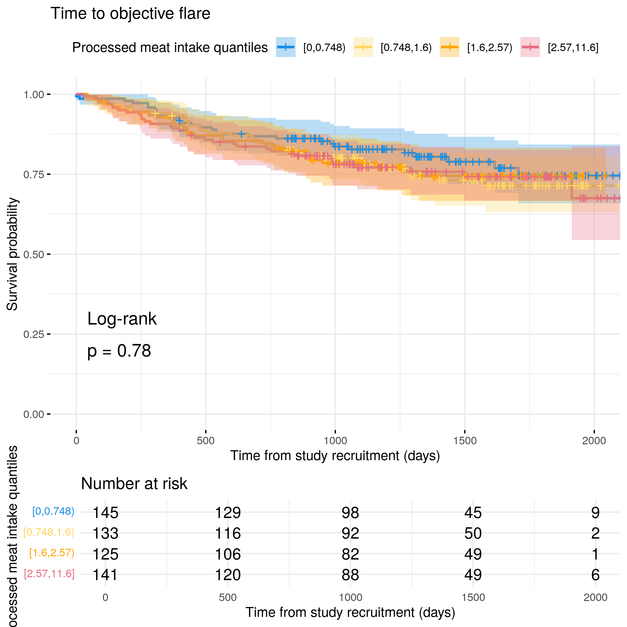
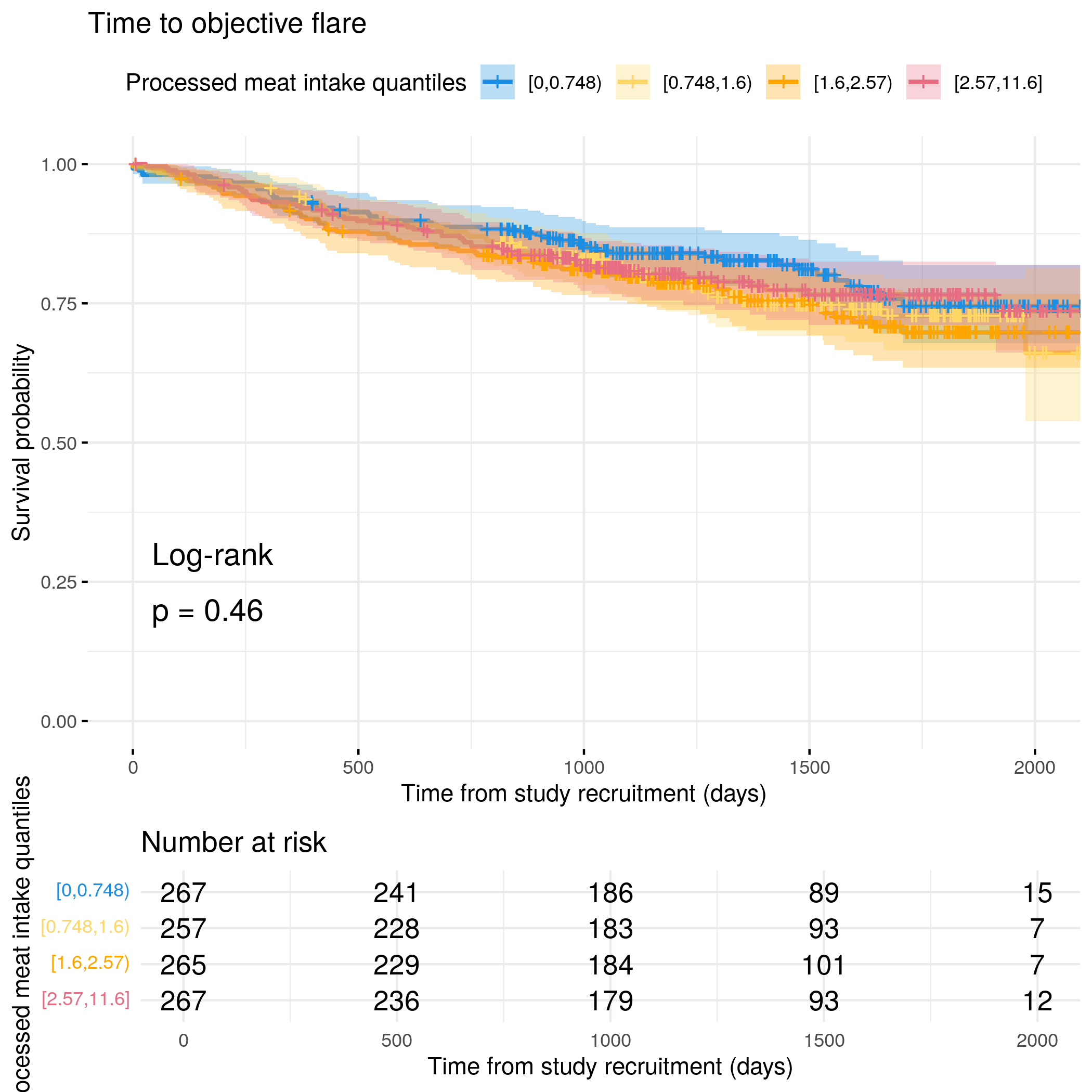
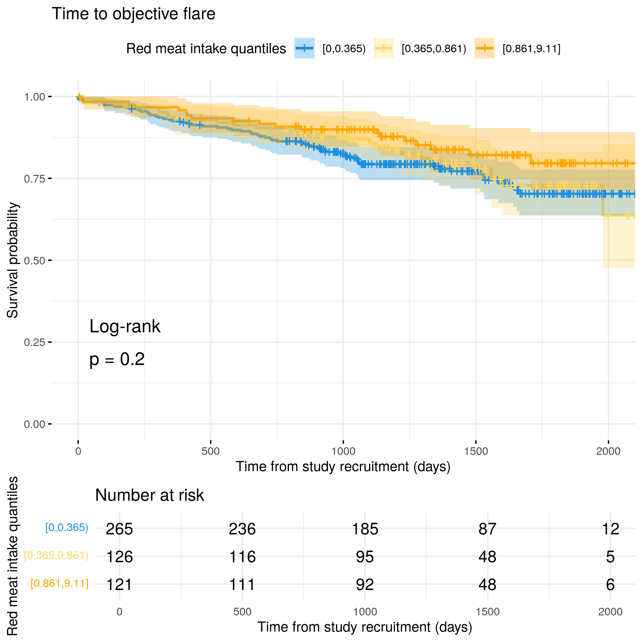
# Categorize processed meat intake by quantilesflare.cd.df<-categorize_by_quantiles(flare.cd.df, "processedMeatIntake", reference_data =flare.df)# Run survival analysis using utility functionanalysis_result<-run_survival_analysis( data =flare.cd.df, var_name ="processedMeatIntake", outcome_time ="softflare_time", outcome_event ="softflare", legend_title ="Processed meat intake quantiles", plot_base_path ="plots/cd/soft-flare/diet/processedMeatIntake", break_time_by =200)# Save plot as RDSsaveRDS(analysis_result$plot, paste0(paths$outdir, "processedMeatIntake-cd-soft.RDS"))# Run Cox model with categorical variablefit.me<-coxph(Surv(softflare_time, softflare)~Sex+cat+IMD+dqi_tot+BMI+processedMeatIntake_cat+frailty(SiteNo), control =coxph.control(outer.max =20), data =flare.cd.df)hrs<-rbind(hrs, broom::tidy(fit.me)|>filter(!grepl("^Sex|^cat|^IMD|^dqi_tot|^BMI|^frailty", term))|>mutate(diagnosis ="CD", flare ="Soft")|>relocate(diagnosis, flare))# Display plot and model summaryknitr::include_graphics("plots/cd/soft-flare/diet/processedMeatIntake.png")
# Run survival analysis using utility function for objective flareanalysis_result<-run_survival_analysis( data =flare.cd.df, var_name ="processedMeatIntake", outcome_time ="hardflare_time", outcome_event ="hardflare", legend_title ="Processed meat intake quantiles", plot_base_path ="plots/cd/hard-flare/diet/processedMeatIntake", break_time_by =500)# Save plot as RDSsaveRDS(analysis_result$plot, paste0(paths$outdir, "processedMeatIntake-cd-hard.RDS"))# Run Cox model with categorical variablefit.me<-coxph(Surv(hardflare_time, hardflare)~Sex+cat+IMD+dqi_tot+BMI+processedMeatIntake_cat+frailty(SiteNo), control =coxph.control(outer.max =20), data =flare.cd.df)hrs<-rbind(hrs, broom::tidy(fit.me)|>filter(!grepl("^Sex|^cat|^IMD|^dqi_tot|^BMI|^frailty", term))|>mutate(diagnosis ="CD", flare ="Hard")|>relocate(diagnosis, flare))# Display plot and model summaryknitr::include_graphics("plots/cd/hard-flare/diet/processedMeatIntake.png")
# Categorize processed meat intake by quantilesflare.uc.df<-categorize_by_quantiles(flare.uc.df, "processedMeatIntake", reference_data =flare.df)# Run survival analysis using utility functionanalysis_result<-run_survival_analysis( data =flare.uc.df, var_name ="processedMeatIntake", outcome_time ="softflare_time", outcome_event ="softflare", legend_title ="Processed meat intake quantiles", plot_base_path ="plots/uc/soft-flare/diet/processedMeatIntake", break_time_by =200)# Save plot as RDSsaveRDS(analysis_result$plot, paste0(paths$outdir, "processedMeatIntake-uc-soft.RDS"))# Run Cox model with categorical variablefit.me<-coxph(Surv(softflare_time, softflare)~Sex+cat+IMD+dqi_tot+BMI+processedMeatIntake_cat+frailty(SiteNo), control =coxph.control(outer.max =20), data =flare.uc.df)hrs<-rbind(hrs, broom::tidy(fit.me)|>filter(!grepl("^Sex|^cat|^IMD|^dqi_tot|^BMI|^frailty", term))|>mutate(diagnosis ="UC", flare ="Soft")|>relocate(diagnosis, flare))# Display plot and model summaryknitr::include_graphics("plots/uc/soft-flare/diet/processedMeatIntake.png")
# Run survival analysis using utility function for objective flareanalysis_result<-run_survival_analysis( data =flare.uc.df, var_name ="processedMeatIntake", outcome_time ="hardflare_time", outcome_event ="hardflare", legend_title ="Processed meat intake quantiles", plot_base_path ="plots/uc/hard-flare/diet/processedMeatIntake", break_time_by =500)# Save plot as RDSsaveRDS(analysis_result$plot, paste0(paths$outdir, "processedMeatIntake-uc-hard.RDS"))# Run Cox model with categorical variablefit.me<-coxph(Surv(hardflare_time, hardflare)~Sex+cat+IMD+dqi_tot+BMI+processedMeatIntake_cat+frailty(SiteNo), control =coxph.control(outer.max =20), data =flare.uc.df)hrs<-rbind(hrs, broom::tidy(fit.me)|>filter(!grepl("^Sex|^cat|^IMD|^dqi_tot|^BMI|^frailty", term))|>mutate(diagnosis ="UC", flare ="Hard")|>relocate(diagnosis, flare))# Display plot and model summaryknitr::include_graphics("plots/uc/hard-flare/diet/processedMeatIntake.png")
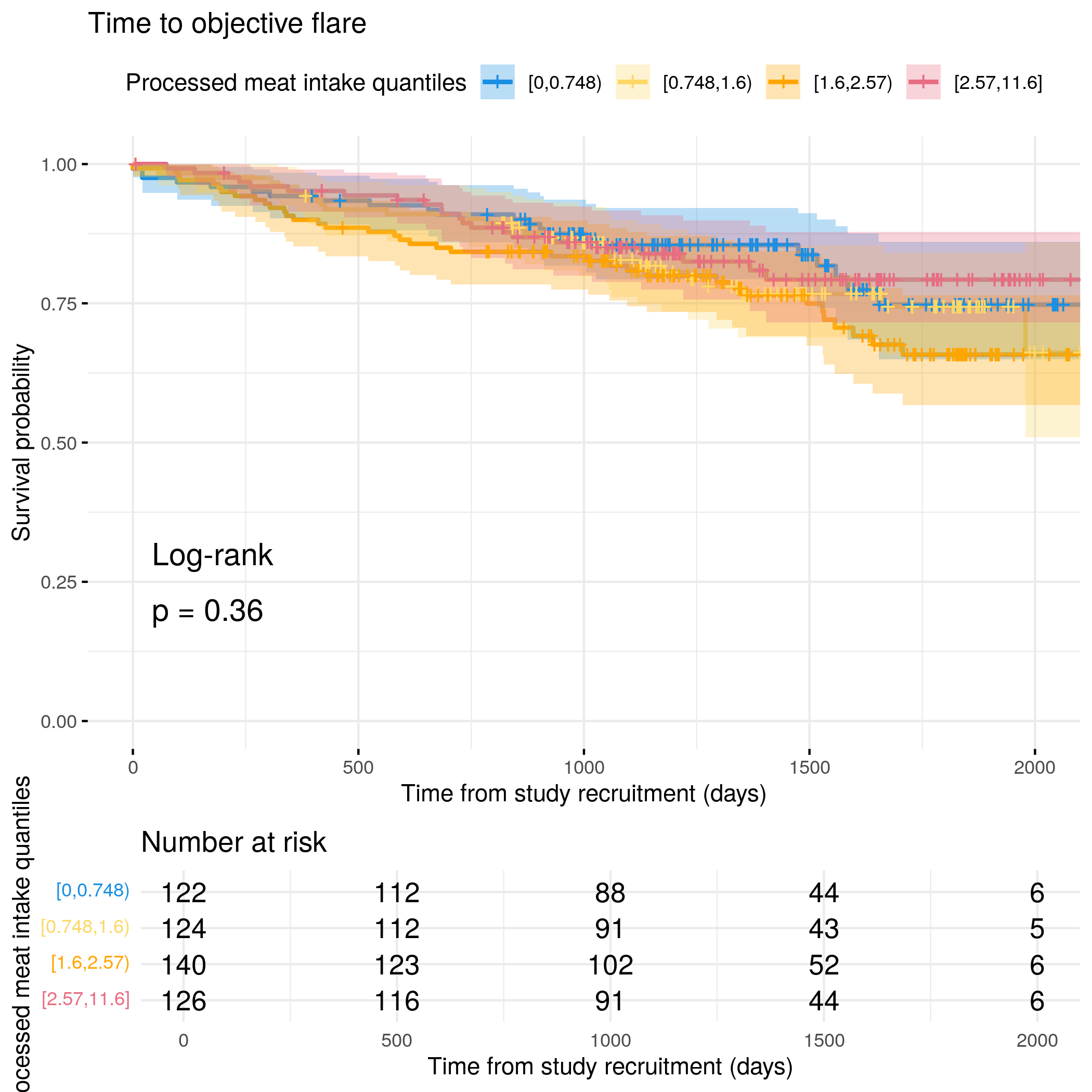
# Run survival analysis using utility function for objective flareanalysis_result<-run_survival_analysis( data =flare.df, var_name ="processedMeatIntake", outcome_time ="hardflare_time", outcome_event ="hardflare", legend_title ="Processed meat intake quantiles", plot_base_path ="plots/ibd/hard-flare/diet/processedMeatIntake", break_time_by =500)# Run Cox model with categorical variablefit.me<-coxph(Surv(hardflare_time, hardflare)~Sex+cat+IMD+dqi_tot+BMI+processedMeatIntake_cat+frailty(SiteNo), control =coxph.control(outer.max =20), data =flare.df)hrs<-rbind(hrs, broom::tidy(fit.me)|>filter(!grepl("^Sex|^cat|^IMD|^dqi_tot|^BMI|^frailty", term))|>mutate(diagnosis ="IBD", flare ="Hard")|>relocate(diagnosis, flare))# Display plot and model summaryknitr::include_graphics("plots/ibd/hard-flare/diet/processedMeatIntake.png")
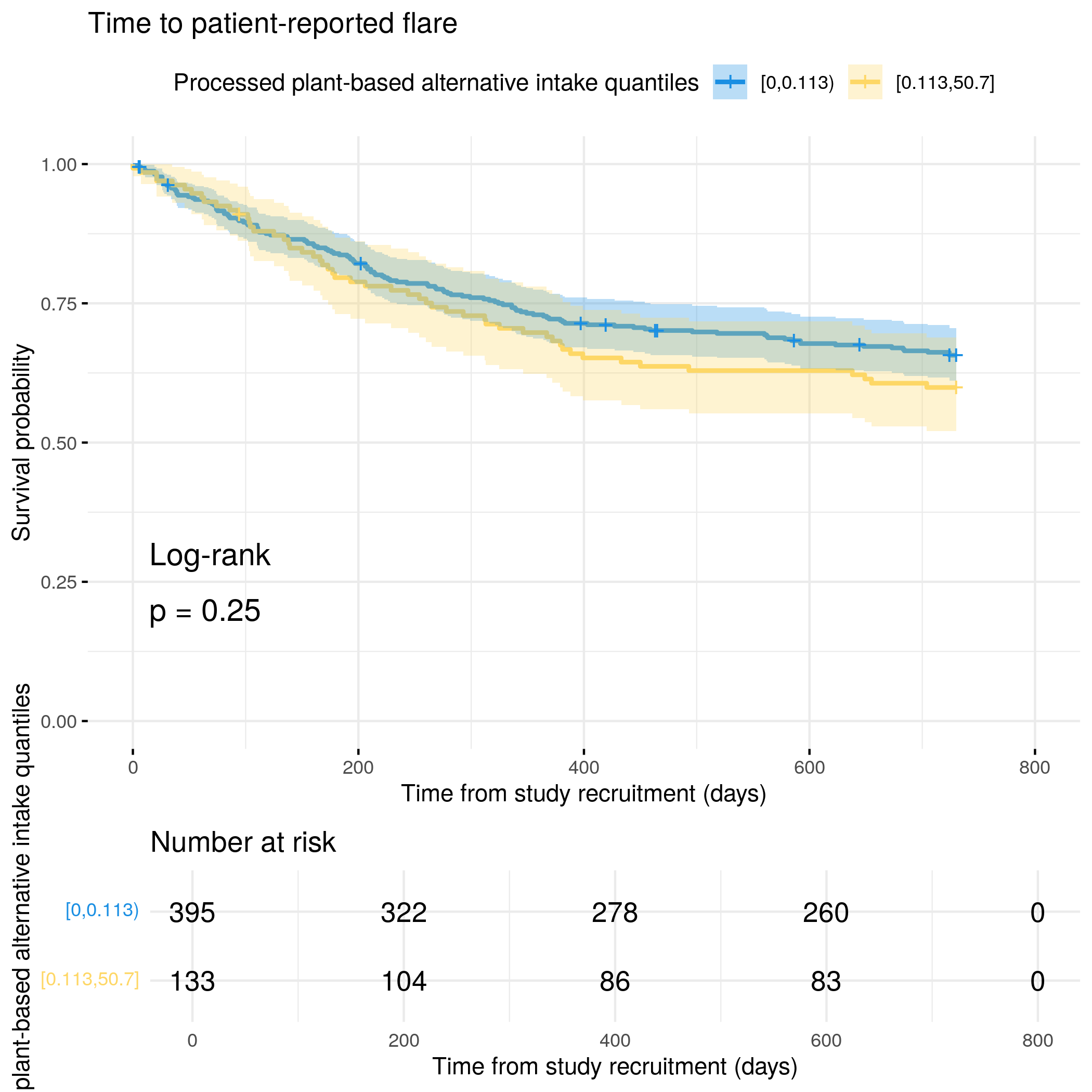
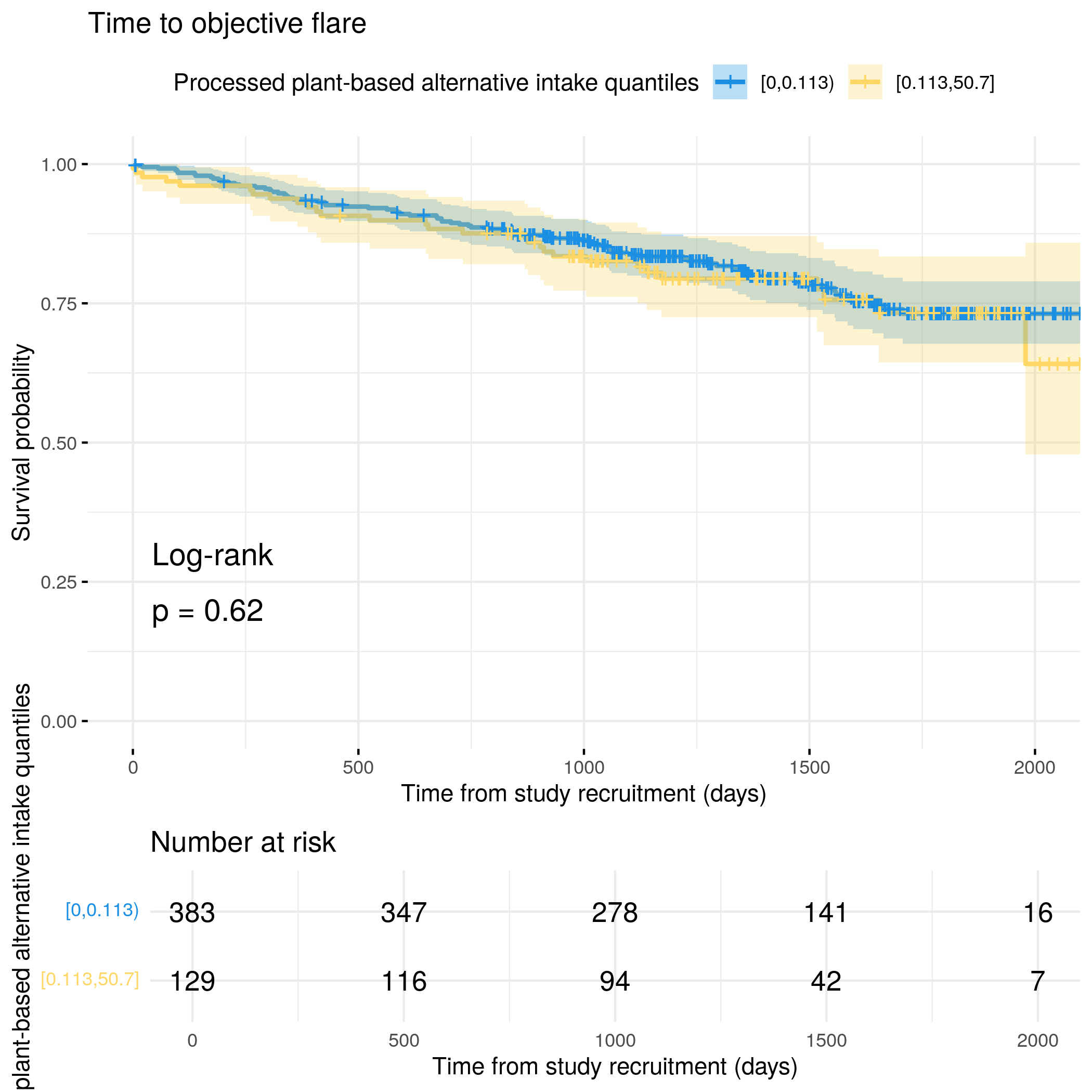
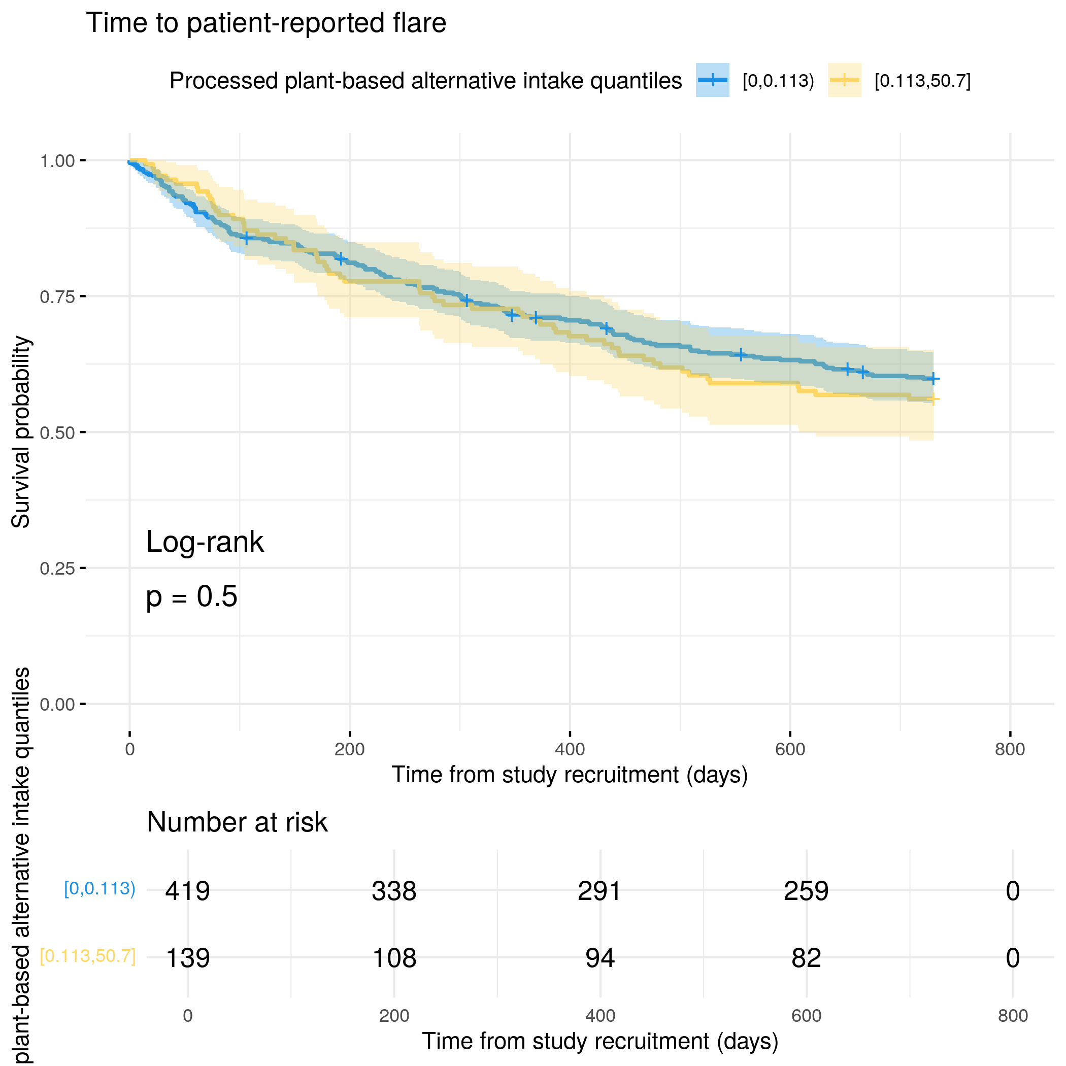
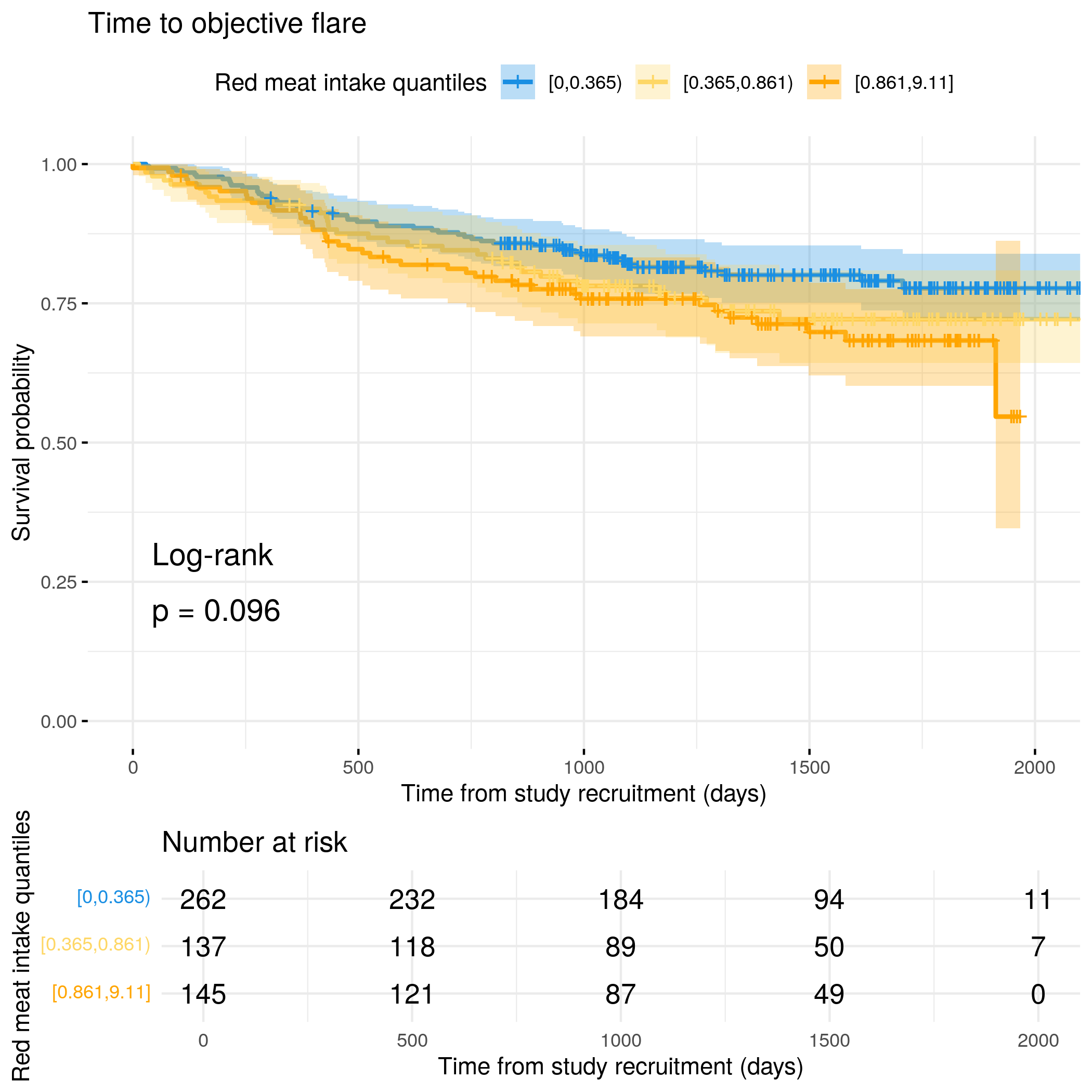
# Categorize processed plant intake by quantilesflare.cd.df<-categorize_by_quantiles(flare.cd.df, "processedPlantIntake", reference_data =flare.df)# Run survival analysis using utility functionanalysis_result<-run_survival_analysis( data =flare.cd.df, var_name ="processedPlantIntake", outcome_time ="softflare_time", outcome_event ="softflare", legend_title ="Processed plant-based alternative intake quantiles", plot_base_path ="plots/cd/soft-flare/diet/processedPlantIntake", break_time_by =200)# Save plot as RDSsaveRDS(analysis_result$plot, paste0(paths$outdir, "processedPlantIntake-cd-soft.RDS"))# Run Cox model with categorical variablefit.me<-coxph(Surv(softflare_time, softflare)~Sex+cat+IMD+dqi_tot+BMI+processedPlantIntake_cat+frailty(SiteNo), control =coxph.control(outer.max =20), data =flare.cd.df)hrs<-rbind(hrs, broom::tidy(fit.me)|>filter(!grepl("^Sex|^cat|^IMD|^dqi_tot|^BMI|^frailty", term))|>mutate(diagnosis ="CD", flare ="Soft")|>relocate(diagnosis, flare))# Display plot and model summaryknitr::include_graphics("plots/cd/soft-flare/diet/processedPlantIntake.png")
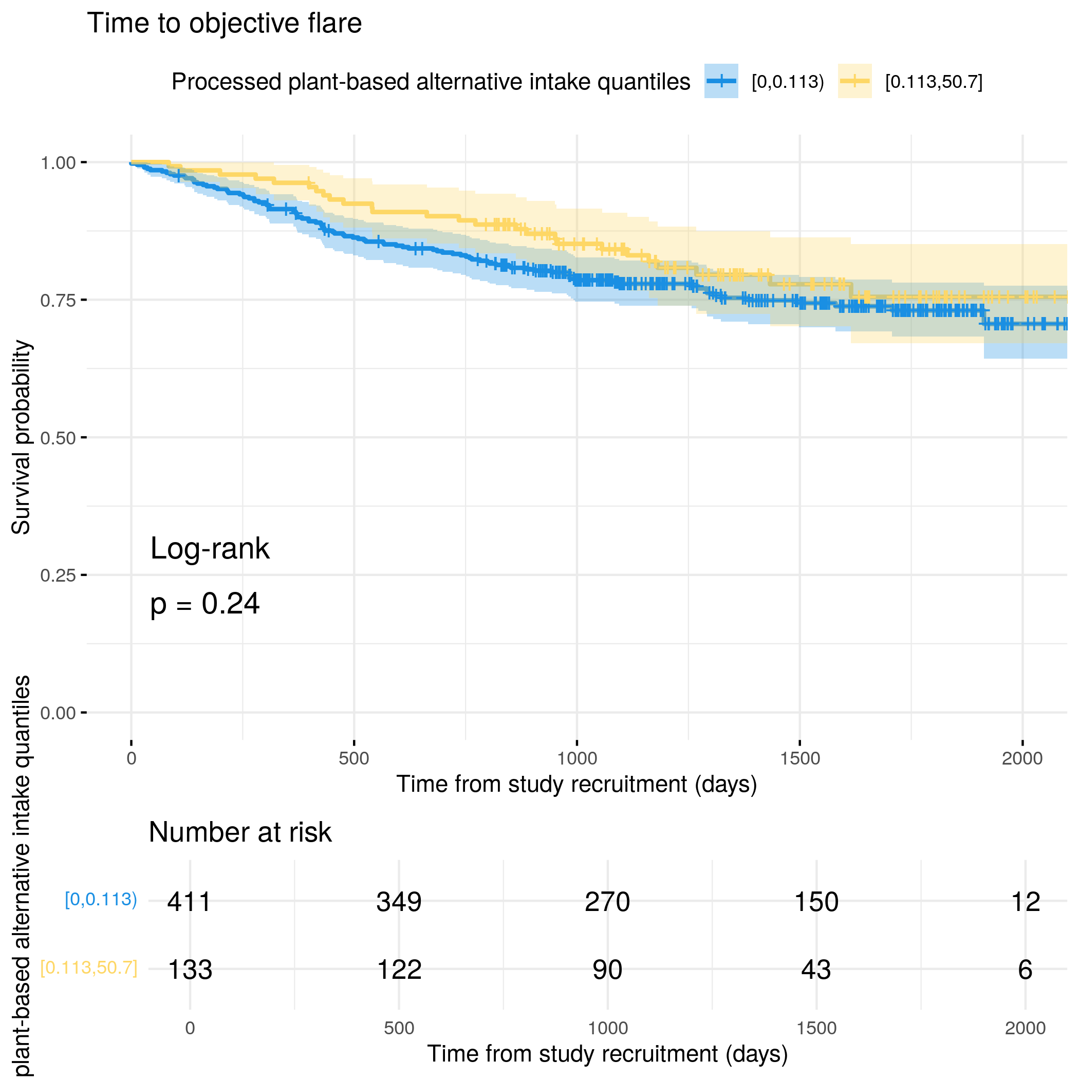
# Run survival analysis using utility function for objective flareanalysis_result<-run_survival_analysis( data =flare.cd.df, var_name ="processedPlantIntake", outcome_time ="hardflare_time", outcome_event ="hardflare", legend_title ="Processed plant-based alternative intake quantiles", plot_base_path ="plots/cd/hard-flare/diet/processedPlantIntake", break_time_by =500)# Save plot as RDSsaveRDS(analysis_result$plot, paste0(paths$outdir, "processedPlantIntake-cd-hard.RDS"))# Run Cox model with categorical variablefit.me<-coxph(Surv(hardflare_time, hardflare)~Sex+cat+IMD+dqi_tot+BMI+processedPlantIntake_cat+frailty(SiteNo), control =coxph.control(outer.max =20), data =flare.cd.df)hrs<-rbind(hrs, broom::tidy(fit.me)|>filter(!grepl("^Sex|^cat|^IMD|^dqi_tot|^BMI|^frailty", term))|>mutate(diagnosis ="CD", flare ="Hard")|>relocate(diagnosis, flare))# Display plot and model summaryknitr::include_graphics("plots/cd/hard-flare/diet/processedPlantIntake.png")
# Categorize processed plant intake by quantilesflare.uc.df<-categorize_by_quantiles(flare.uc.df, "processedPlantIntake", reference_data =flare.df)# Run survival analysis using utility functionanalysis_result<-run_survival_analysis( data =flare.uc.df, var_name ="processedPlantIntake", outcome_time ="softflare_time", outcome_event ="softflare", legend_title ="Processed plant-based alternative intake quantiles", plot_base_path ="plots/uc/soft-flare/diet/processedPlantIntake", break_time_by =200)# Save plot as RDSsaveRDS(analysis_result$plot, paste0(paths$outdir, "processedPlantIntake-uc-soft.RDS"))# Run Cox model with categorical variablefit.me<-coxph(Surv(softflare_time, softflare)~Sex+cat+IMD+dqi_tot+BMI+processedPlantIntake_cat+frailty(SiteNo), control =coxph.control(outer.max =20), data =flare.uc.df)hrs<-rbind(hrs, broom::tidy(fit.me)|>filter(!grepl("^Sex|^cat|^IMD|^dqi_tot|^BMI|^frailty", term))|>mutate(diagnosis ="UC", flare ="Soft")|>relocate(diagnosis, flare))# Display plot and model summaryknitr::include_graphics("plots/uc/soft-flare/diet/processedPlantIntake.png")
# Run survival analysis using utility function for objective flareanalysis_result<-run_survival_analysis( data =flare.uc.df, var_name ="processedPlantIntake", outcome_time ="hardflare_time", outcome_event ="hardflare", legend_title ="Processed plant-based alternative intake quantiles", plot_base_path ="plots/uc/hard-flare/diet/processedPlantIntake", break_time_by =500)# Save plot as RDSsaveRDS(analysis_result$plot, paste0(paths$outdir, "processedPlantIntake-uc-hard.RDS"))# Run Cox model with categorical variablefit.me<-coxph(Surv(hardflare_time, hardflare)~Sex+cat+IMD+dqi_tot+BMI+processedPlantIntake_cat+frailty(SiteNo), control =coxph.control(outer.max =20), data =flare.uc.df)hrs<-rbind(hrs, broom::tidy(fit.me)|>filter(!grepl("^Sex|^cat|^IMD|^dqi_tot|^BMI|^frailty", term))|>mutate(diagnosis ="UC", flare ="Hard")|>relocate(diagnosis, flare))# Display plot and model summaryknitr::include_graphics("plots/uc/hard-flare/diet/processedPlantIntake.png")
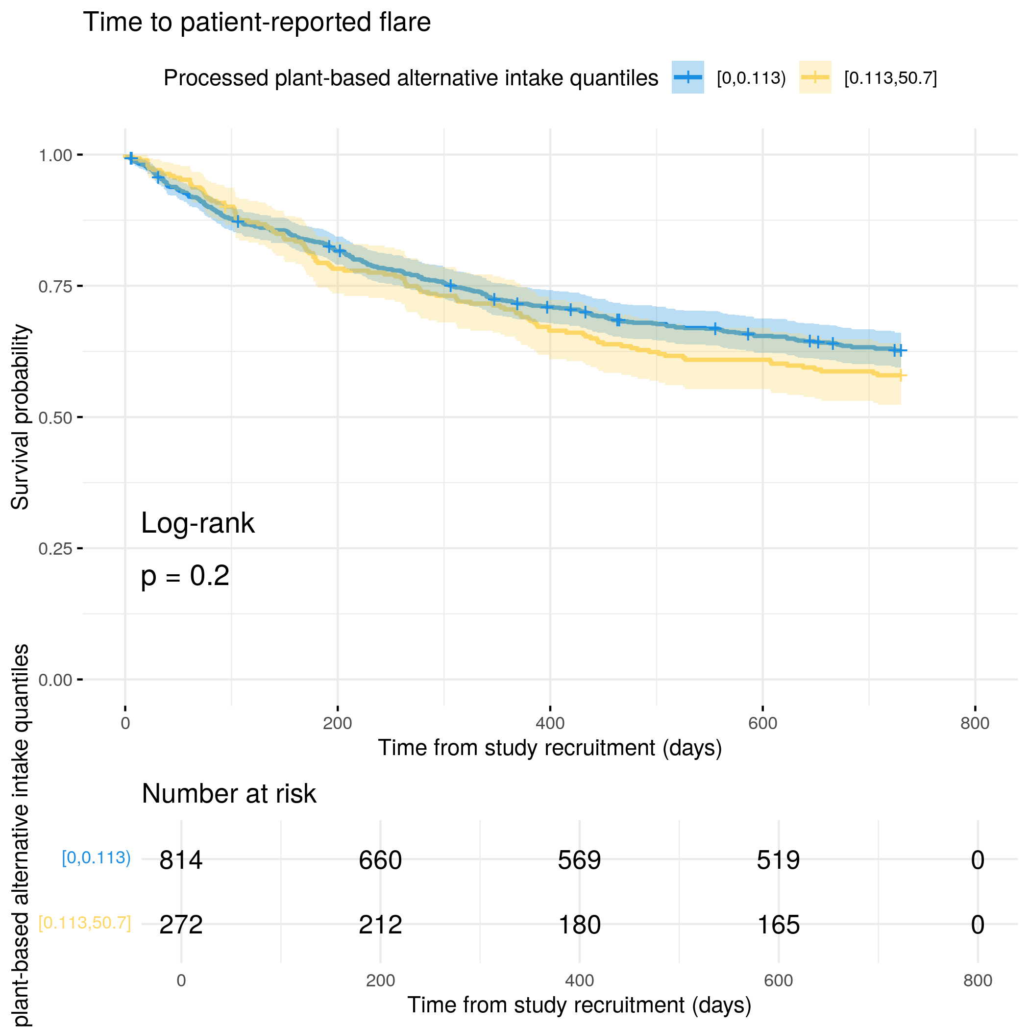
# Categorize processed plant intake by quantilesflare.df<-categorize_by_quantiles(flare.df, "processedPlantIntake", reference_data =flare.df)# Run survival analysis using utility functionanalysis_result<-run_survival_analysis( data =flare.df, var_name ="processedPlantIntake", outcome_time ="softflare_time", outcome_event ="softflare", legend_title ="Processed plant-based alternative intake quantiles", plot_base_path ="plots/ibd/soft-flare/diet/processedPlantIntake", break_time_by =200)# Run Cox model with categorical variablefit.me<-coxph(Surv(softflare_time, softflare)~Sex+cat+IMD+dqi_tot+BMI+processedPlantIntake_cat+frailty(SiteNo), control =coxph.control(outer.max =20), data =flare.df)hrs<-rbind(hrs, broom::tidy(fit.me)|>filter(!grepl("^Sex|^cat|^IMD|^dqi_tot|^BMI|^frailty", term))|>mutate(diagnosis ="IBD", flare ="Soft")|>relocate(diagnosis, flare))# Display plot and model summaryknitr::include_graphics("plots/ibd/soft-flare/diet/processedPlantIntake.png")
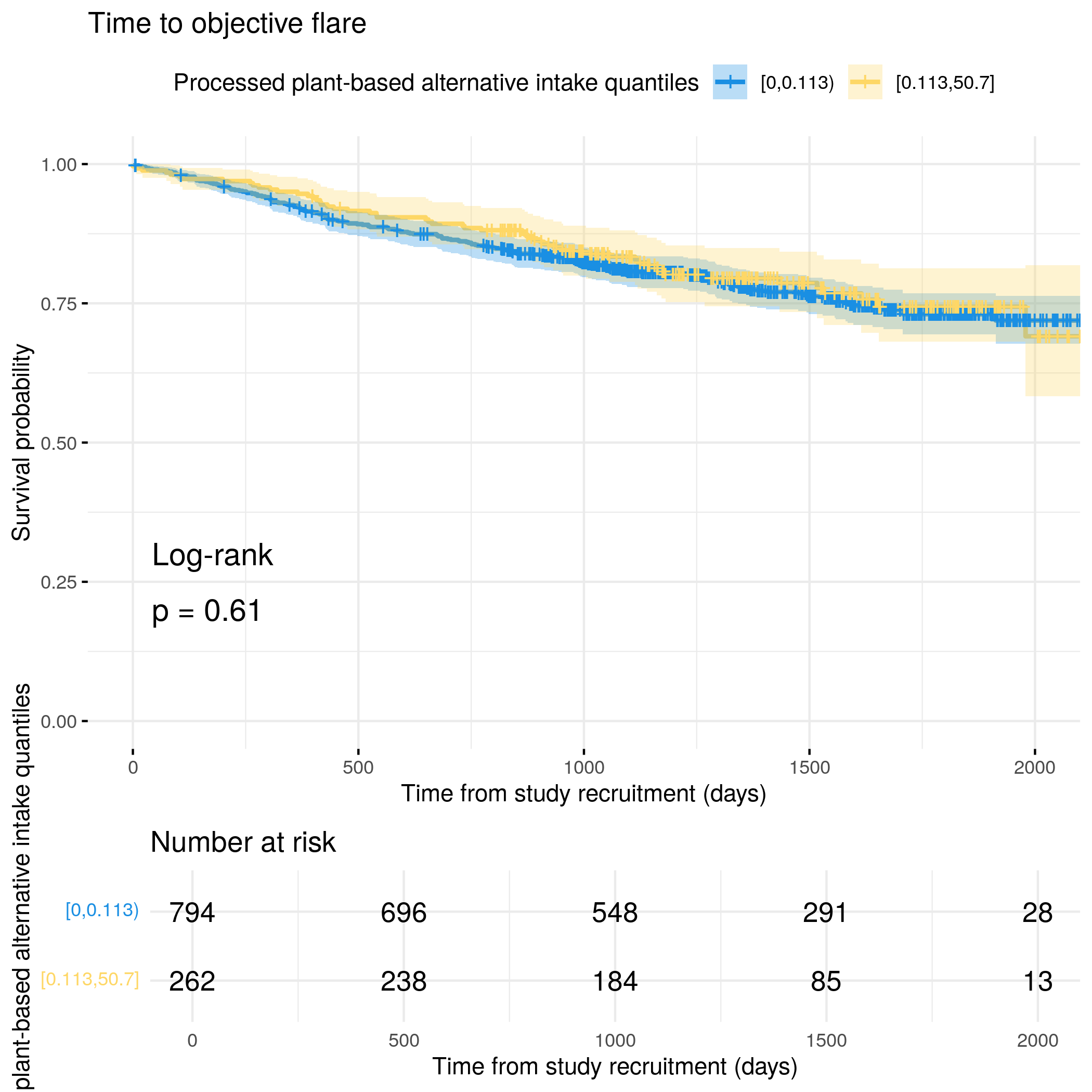
# Run survival analysis using utility function for objective flareanalysis_result<-run_survival_analysis( data =flare.df, var_name ="processedPlantIntake", outcome_time ="hardflare_time", outcome_event ="hardflare", legend_title ="Processed plant-based alternative intake quantiles", plot_base_path ="plots/ibd/hard-flare/diet/processedPlantIntake", break_time_by =500)# Run Cox model with categorical variablefit.me<-coxph(Surv(hardflare_time, hardflare)~Sex+cat+IMD+dqi_tot+BMI+processedPlantIntake_cat+frailty(SiteNo), control =coxph.control(outer.max =20), data =flare.df)hrs<-rbind(hrs, broom::tidy(fit.me)|>filter(!grepl("^Sex|^cat|^IMD|^dqi_tot|^BMI|^frailty", term))|>mutate(diagnosis ="IBD", flare ="Hard")|>relocate(diagnosis, flare))# Display plot and model summaryknitr::include_graphics("plots/ibd/hard-flare/diet/processedPlantIntake.png")
# Categorize fruit intake by quantilesflare.cd.df<-categorize_by_quantiles(flare.cd.df, "fruitIntake", reference_data =flare.df)# Run survival analysis using utility functionanalysis_result<-run_survival_analysis( data =flare.cd.df, var_name ="fruitIntake", outcome_time ="softflare_time", outcome_event ="softflare", legend_title ="Fruit intake quantiles", plot_base_path ="plots/cd/soft-flare/diet/fruitIntake", break_time_by =200)# Save plot as RDSsaveRDS(analysis_result$plot, paste0(paths$outdir, "fruitIntake-cd-soft.RDS"))# Run Cox model with categorical variablefit.me<-coxph(Surv(softflare_time, softflare)~Sex+cat+IMD+dqi_tot+BMI+fruitIntake_cat+frailty(SiteNo), control =coxph.control(outer.max =20), data =flare.cd.df)hrs<-rbind(hrs, broom::tidy(fit.me)|>filter(!grepl("^Sex|^cat|^IMD|^dqi_tot|^BMI|^frailty", term))|>mutate(diagnosis ="CD", flare ="Soft")|>relocate(diagnosis, flare))# Display plot and model summaryknitr::include_graphics("plots/cd/soft-flare/diet/fruitIntake.png")
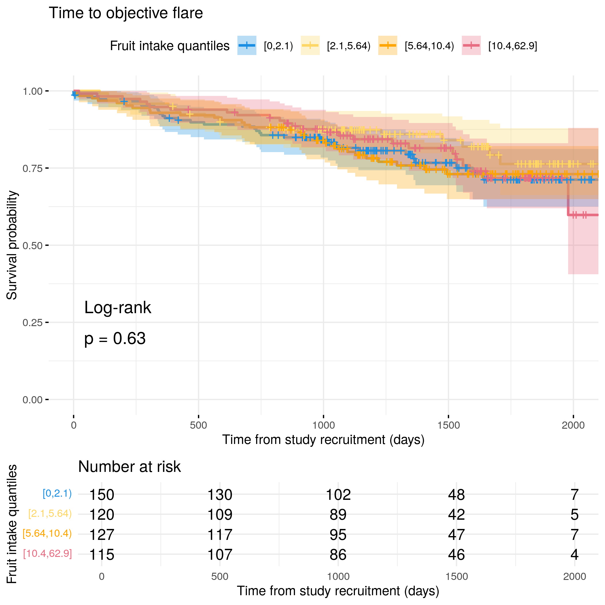
# Run survival analysis using utility function for objective flareanalysis_result<-run_survival_analysis( data =flare.cd.df, var_name ="fruitIntake", outcome_time ="hardflare_time", outcome_event ="hardflare", legend_title ="Fruit intake quantiles", plot_base_path ="plots/cd/hard-flare/diet/fruitIntake", break_time_by =500)# Save plot as RDSsaveRDS(analysis_result$plot, paste0(paths$outdir, "fruitIntake-cd-hard.RDS"))# Run Cox model with categorical variablefit.me<-coxph(Surv(hardflare_time, hardflare)~Sex+cat+IMD+dqi_tot+BMI+fruitIntake_cat+frailty(SiteNo), control =coxph.control(outer.max =20), data =flare.cd.df)hrs<-rbind(hrs, broom::tidy(fit.me)|>filter(!grepl("^Sex|^cat|^IMD|^dqi_tot|^BMI|^frailty", term))|>mutate(diagnosis ="CD", flare ="Hard")|>relocate(diagnosis, flare))# Display plot and model summaryknitr::include_graphics("plots/cd/hard-flare/diet/fruitIntake.png")
# Categorize fruit intake by quantilesflare.uc.df<-categorize_by_quantiles(flare.uc.df, "fruitIntake", reference_data =flare.df)# Run survival analysis using utility functionanalysis_result<-run_survival_analysis( data =flare.uc.df, var_name ="fruitIntake", outcome_time ="softflare_time", outcome_event ="softflare", legend_title ="Fruit intake quantiles", plot_base_path ="plots/uc/soft-flare/diet/fruitIntake", break_time_by =200)# Save plot as RDSsaveRDS(analysis_result$plot, paste0(paths$outdir, "fruitIntake-uc-soft.RDS"))# Run Cox model with categorical variablefit.me<-coxph(Surv(softflare_time, softflare)~Sex+cat+IMD+dqi_tot+BMI+fruitIntake_cat+frailty(SiteNo), control =coxph.control(outer.max =20), data =flare.uc.df)hrs<-rbind(hrs, broom::tidy(fit.me)|>filter(!grepl("^Sex|^cat|^IMD|^dqi_tot|^BMI|^frailty", term))|>mutate(diagnosis ="UC", flare ="Soft")|>relocate(diagnosis, flare))# Display plot and model summaryknitr::include_graphics("plots/uc/soft-flare/diet/fruitIntake.png")
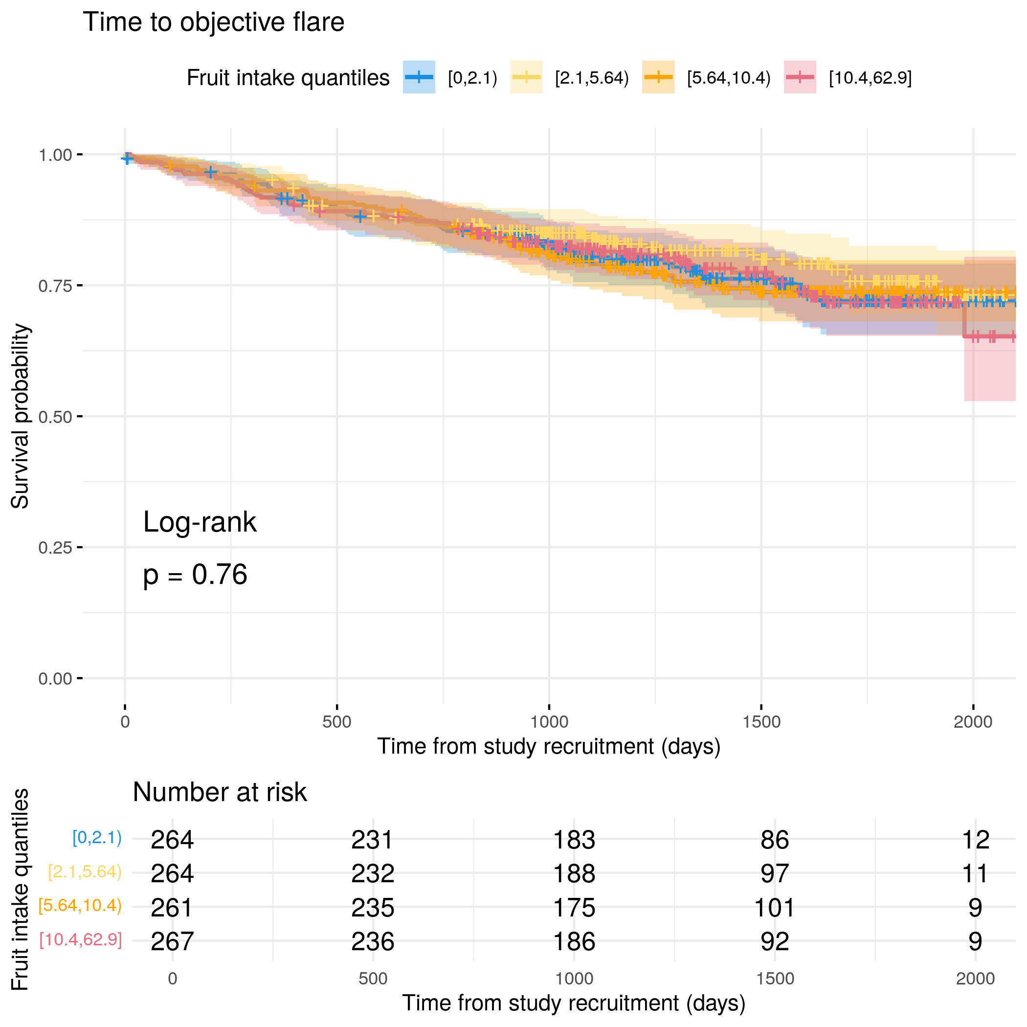
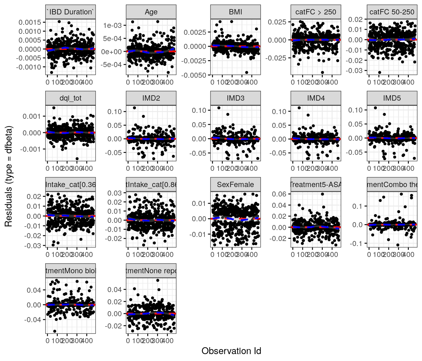
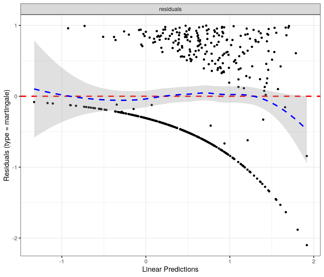
# Run survival analysis using utility function for objective flareanalysis_result<-run_survival_analysis( data =flare.uc.df, var_name ="fruitIntake", outcome_time ="hardflare_time", outcome_event ="hardflare", legend_title ="Fruit intake quantiles", plot_base_path ="plots/uc/hard-flare/diet/fruitIntake", break_time_by =500)# Save plot as RDSsaveRDS(analysis_result$plot, paste0(paths$outdir, "fruitIntake-uc-hard.RDS"))# Run Cox model with categorical variablefit.me<-coxph(Surv(hardflare_time, hardflare)~Sex+cat+IMD+fruitIntake_cat+dqi_tot+BMI+frailty(SiteNo), control =coxph.control(outer.max =20), data =flare.uc.df)hrs<-rbind(hrs, broom::tidy(fit.me)|>filter(!grepl("^Sex|^cat|^IMD|^dqi_tot|^BMI|^frailty", term))|>mutate(diagnosis ="UC", flare ="Hard")|>relocate(diagnosis, flare))# Display plot and model summaryknitr::include_graphics("plots/uc/hard-flare/diet/fruitIntake.png")
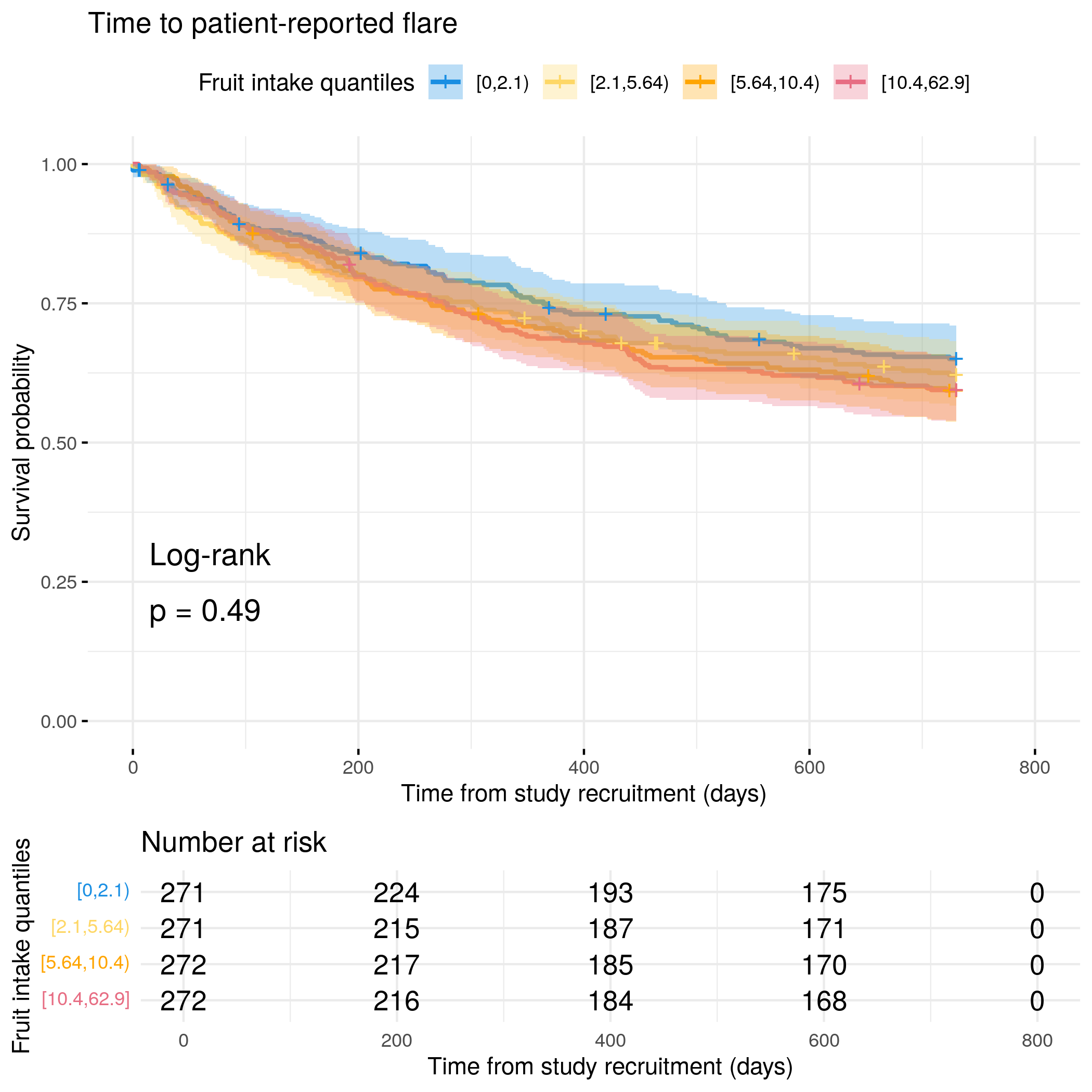
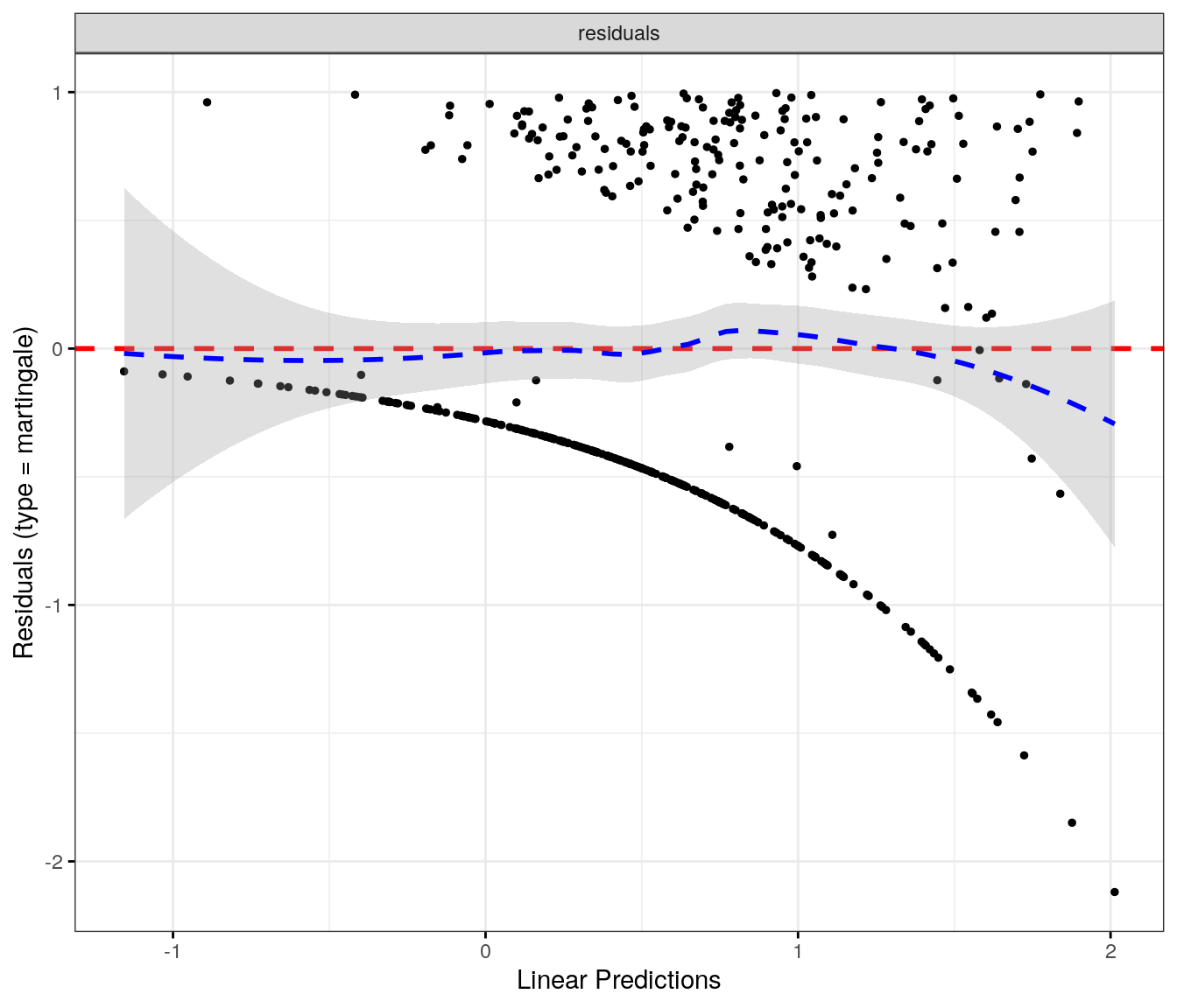
# Categorize fruit intake by quantilesflare.df<-categorize_by_quantiles(flare.df, "fruitIntake", reference_data =flare.df)# Run survival analysis using utility functionanalysis_result<-run_survival_analysis( data =flare.df, var_name ="fruitIntake", outcome_time ="softflare_time", outcome_event ="softflare", legend_title ="Fruit intake quantiles", plot_base_path ="plots/ibd/soft-flare/diet/fruitIntake", break_time_by =200)# Run Cox model with categorical variablefit.me<-coxph(Surv(softflare_time, softflare)~Sex+cat+IMD+dqi_tot+BMI+fruitIntake_cat+frailty(SiteNo), control =coxph.control(outer.max =20), data =flare.df)hrs<-rbind(hrs, broom::tidy(fit.me)|>filter(!grepl("^Sex|^cat|^IMD|^dqi_tot|^BMI|^frailty", term))|>mutate(diagnosis ="IBD", flare ="Soft")|>relocate(diagnosis, flare))# Display plot and model summaryknitr::include_graphics("plots/ibd/soft-flare/diet/fruitIntake.png")
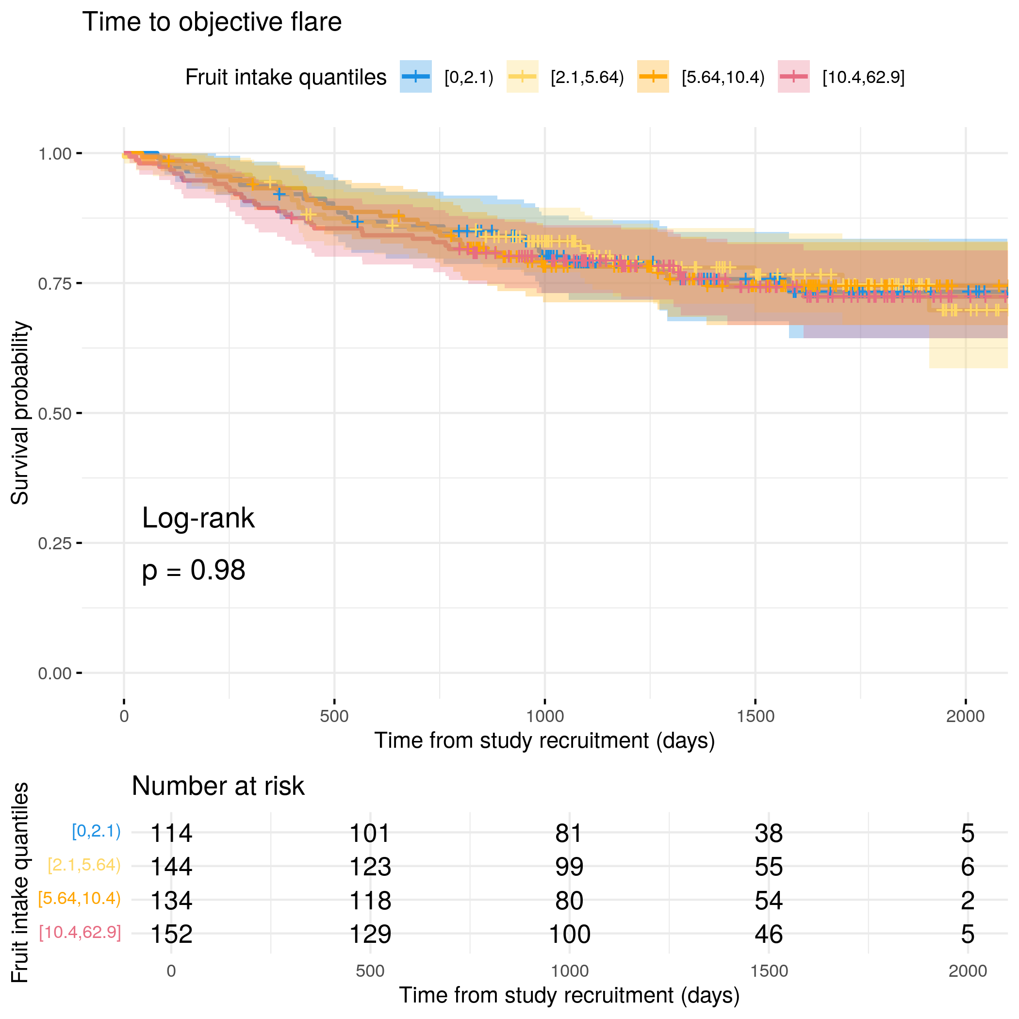
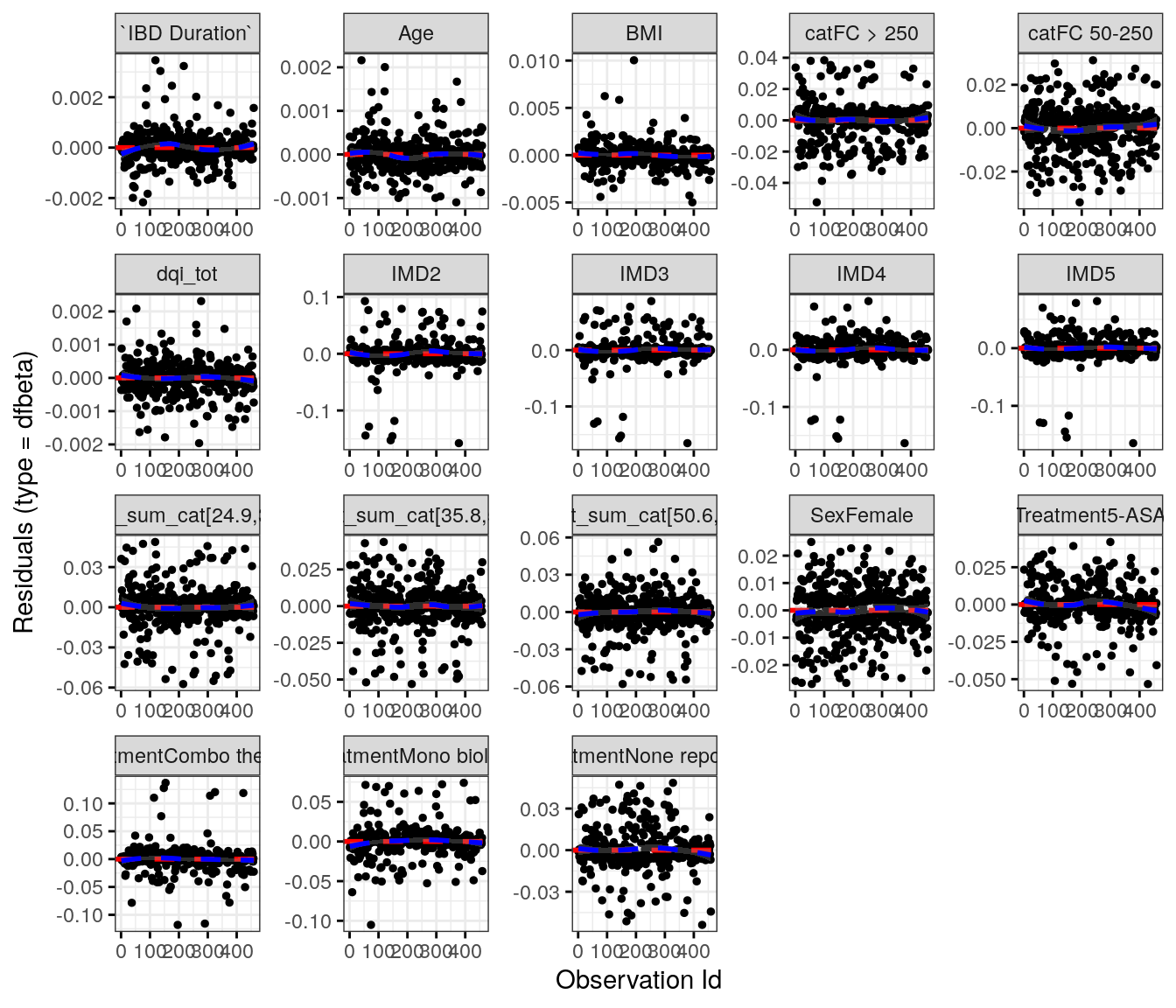
# Run survival analysis using utility function for objective flareanalysis_result<-run_survival_analysis( data =flare.df, var_name ="fruitIntake", outcome_time ="hardflare_time", outcome_event ="hardflare", legend_title ="Fruit intake quantiles", plot_base_path ="plots/ibd/hard-flare/diet/fruitIntake", break_time_by =500)# Run Cox model with categorical variablefit.me<-coxph(Surv(hardflare_time, hardflare)~Sex+cat+IMD+dqi_tot+BMI+fruitIntake_cat+frailty(SiteNo), control =coxph.control(outer.max =20), data =flare.df)hrs<-rbind(hrs, broom::tidy(fit.me)|>filter(!grepl("^Sex|^cat|^IMD|^dqi_tot|^BMI|^frailty", term))|>mutate(diagnosis ="IBD", flare ="Hard")|>relocate(diagnosis, flare))# Display plot and model summaryknitr::include_graphics("plots/ibd/hard-flare/diet/fruitIntake.png")
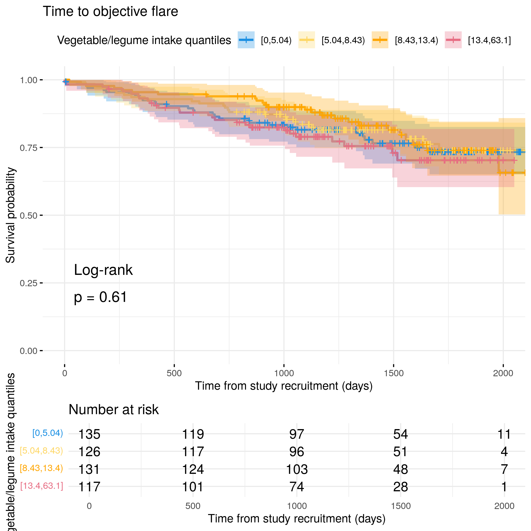
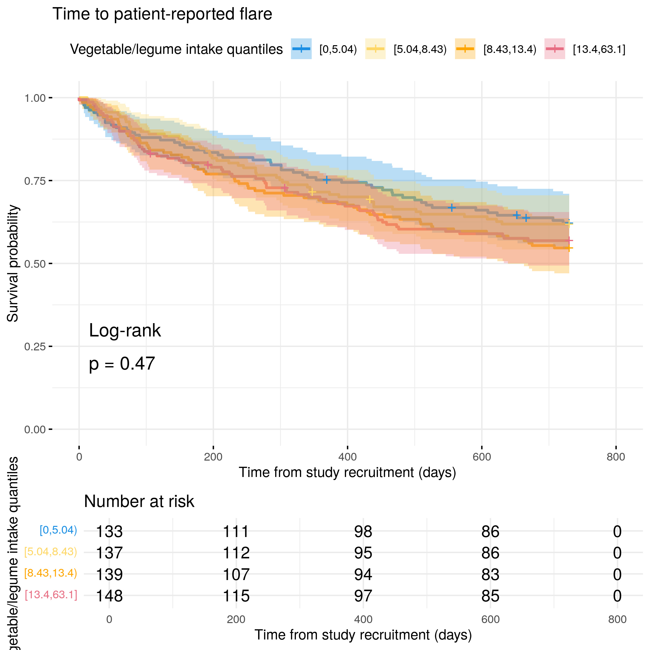
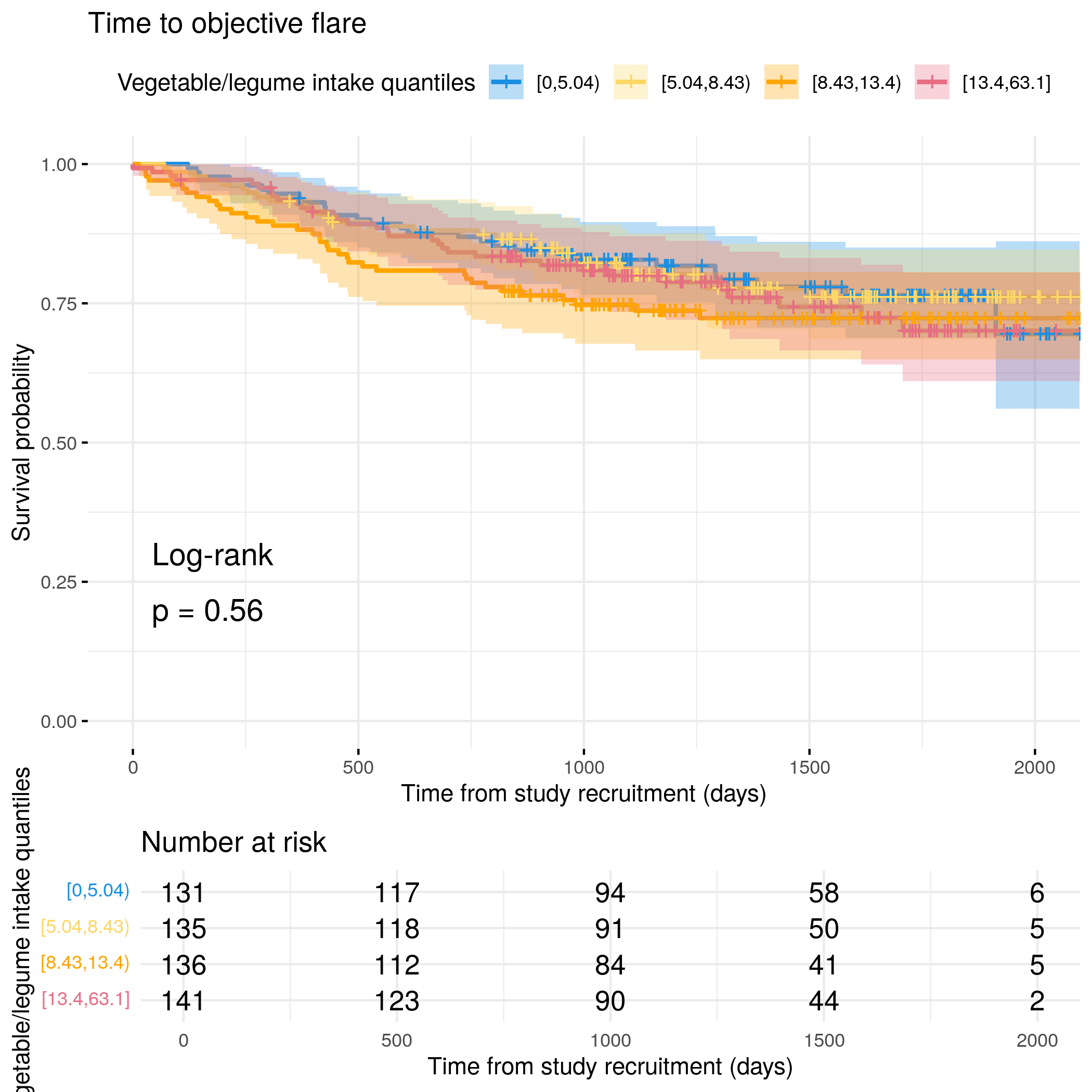
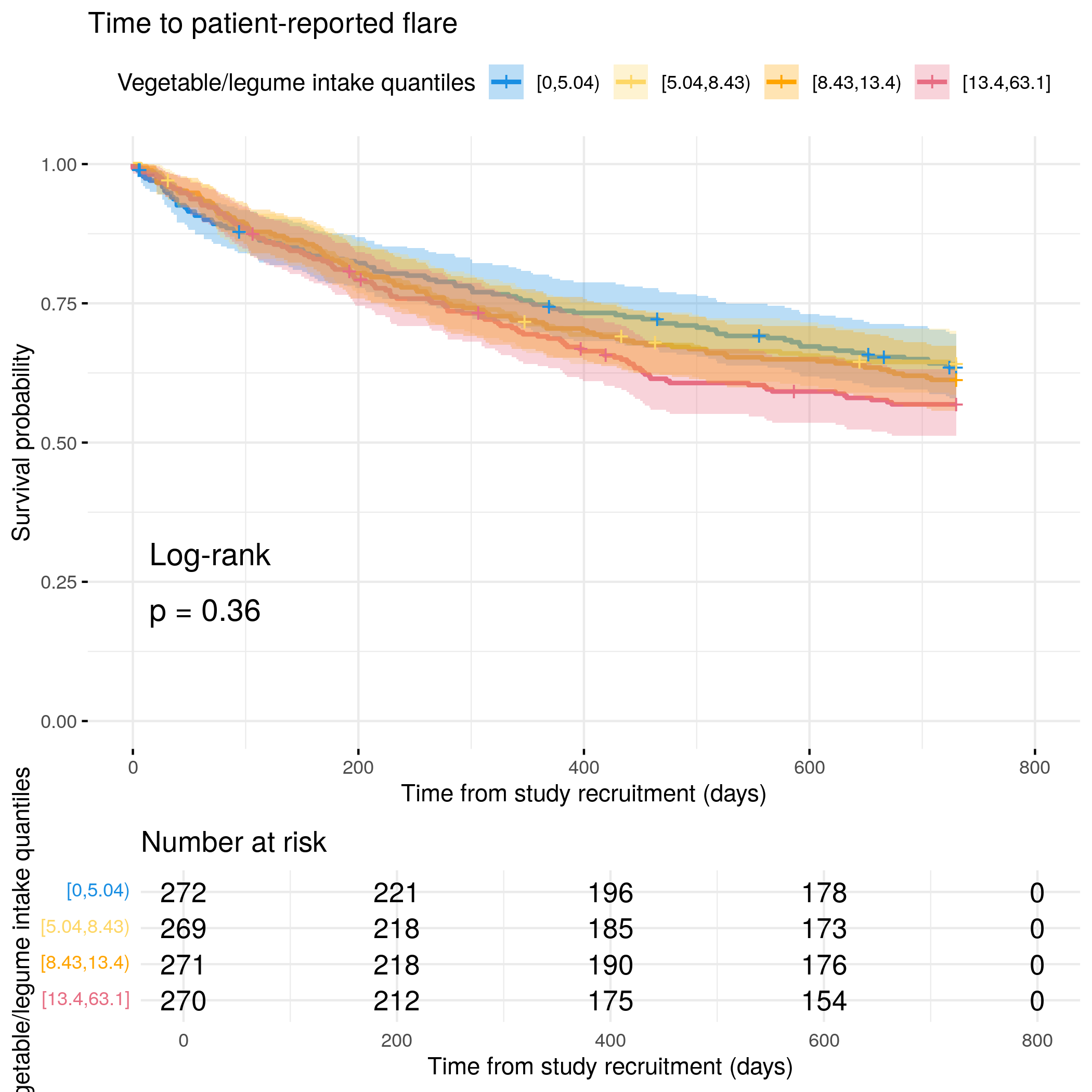
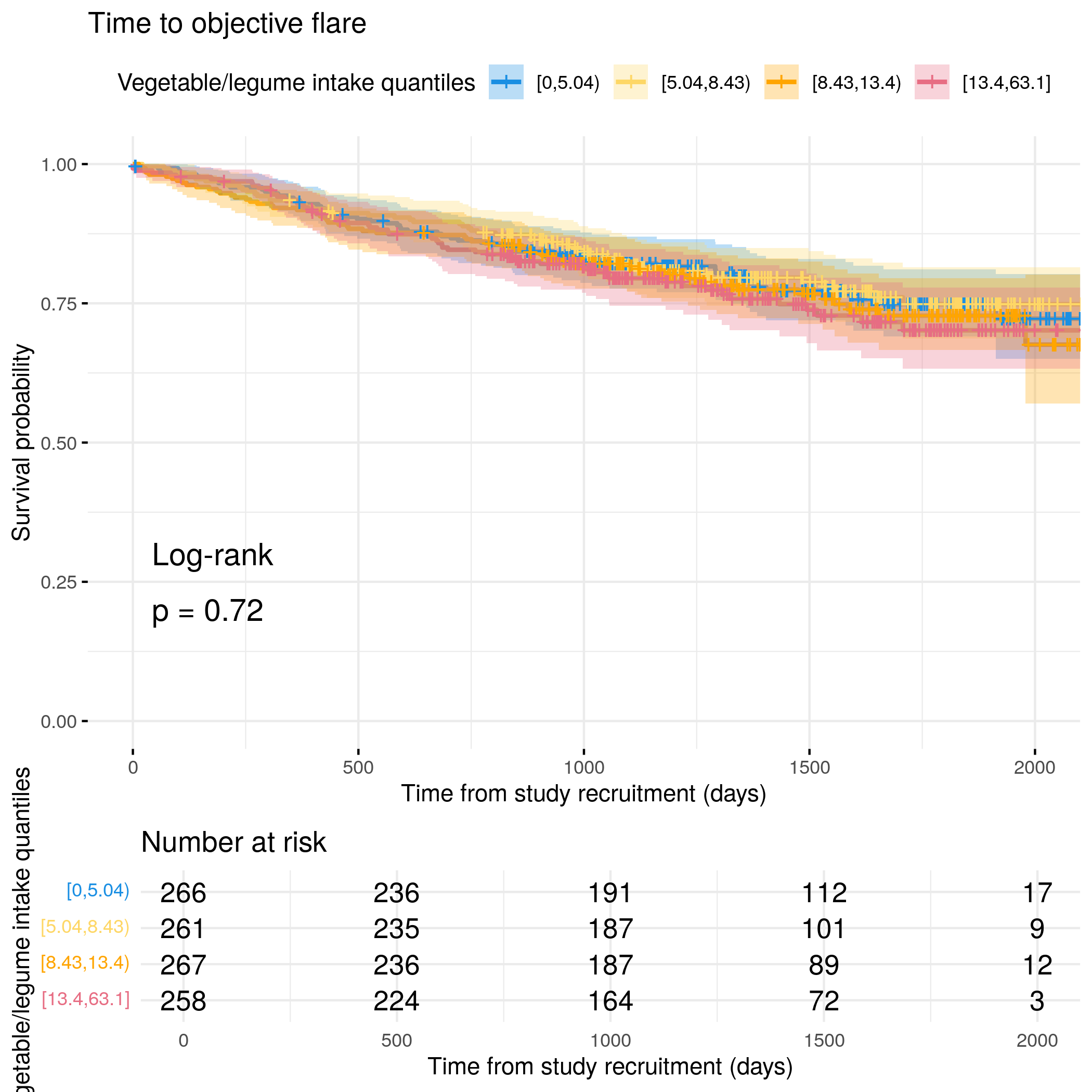
# Categorize vegetable intake by quantilesflare.cd.df<-categorize_by_quantiles(flare.cd.df, "vegIntake", reference_data =flare.df)# Run survival analysis using utility functionanalysis_result<-run_survival_analysis( data =flare.cd.df, var_name ="vegIntake", outcome_time ="softflare_time", outcome_event ="softflare", legend_title ="Vegetable/legume intake quantiles", plot_base_path ="plots/cd/soft-flare/diet/vegIntake", break_time_by =200)# Save plot as RDSsaveRDS(analysis_result$plot, paste0(paths$outdir, "vegIntake-cd-soft.RDS"))# Run Cox model with categorical variablefit.me<-coxph(Surv(softflare_time, softflare)~Sex+cat+IMD+dqi_tot+BMI+vegIntake_cat+frailty(SiteNo), control =coxph.control(outer.max =20), data =flare.cd.df)hrs<-rbind(hrs, broom::tidy(fit.me)|>filter(!grepl("^Sex|^cat|^IMD|^dqi_tot|^BMI|^frailty", term))|>mutate(diagnosis ="CD", flare ="Soft")|>relocate(diagnosis, flare))# Display plot and model summaryknitr::include_graphics("plots/cd/soft-flare/diet/vegIntake.png")
# Run survival analysis using utility function for objective flareanalysis_result<-run_survival_analysis( data =flare.cd.df, var_name ="vegIntake", outcome_time ="hardflare_time", outcome_event ="hardflare", legend_title ="Vegetable/legume intake quantiles", plot_base_path ="plots/cd/hard-flare/diet/vegIntake", break_time_by =500)# Save plot as RDSsaveRDS(analysis_result$plot, paste0(paths$outdir, "vegIntake-cd-hard.RDS"))# Run Cox model with categorical variablefit.me<-coxph(Surv(hardflare_time, hardflare)~Sex+cat+IMD+dqi_tot+BMI+vegIntake_cat+frailty(SiteNo), control =coxph.control(outer.max =20), data =flare.cd.df)hrs<-rbind(hrs, broom::tidy(fit.me)|>filter(!grepl("^Sex|^cat|^IMD|^dqi_tot|^BMI|^frailty", term))|>mutate(diagnosis ="CD", flare ="Hard")|>relocate(diagnosis, flare))# Display plot and model summaryknitr::include_graphics("plots/cd/hard-flare/diet/vegIntake.png")
# Categorize vegetable intake by quantilesflare.uc.df<-categorize_by_quantiles(flare.uc.df, "vegIntake", reference_data =flare.df)# Run survival analysis using utility functionanalysis_result<-run_survival_analysis( data =flare.uc.df, var_name ="vegIntake", outcome_time ="softflare_time", outcome_event ="softflare", legend_title ="Vegetable/legume intake quantiles", plot_base_path ="plots/uc/soft-flare/diet/vegIntake", break_time_by =200)# Save plot as RDSsaveRDS(analysis_result$plot, paste0(paths$outdir, "vegIntake-uc-soft.RDS"))# Run Cox model with categorical variablefit.me<-coxph(Surv(softflare_time, softflare)~Sex+cat+IMD+dqi_tot+BMI+vegIntake_cat+frailty(SiteNo), control =coxph.control(outer.max =20), data =flare.uc.df)hrs<-rbind(hrs, broom::tidy(fit.me)|>filter(!grepl("^Sex|^cat|^IMD|^dqi_tot|^BMI|^frailty", term))|>mutate(diagnosis ="UC", flare ="Soft")|>relocate(diagnosis, flare))# Display plot and model summaryknitr::include_graphics("plots/uc/soft-flare/diet/vegIntake.png")
# Run survival analysis using utility function for objective flareanalysis_result<-run_survival_analysis( data =flare.uc.df, var_name ="vegIntake", outcome_time ="hardflare_time", outcome_event ="hardflare", legend_title ="Vegetable/legume intake quantiles", plot_base_path ="plots/uc/hard-flare/diet/vegIntake", break_time_by =500)# Save plot as RDSsaveRDS(analysis_result$plot, paste0(paths$outdir, "vegIntake-uc-hard.RDS"))# Run Cox model with categorical variablefit.me<-coxph(Surv(hardflare_time, hardflare)~Sex+cat+IMD+dqi_tot+BMI+vegIntake_cat+frailty(SiteNo), control =coxph.control(outer.max =20), data =flare.uc.df)hrs<-rbind(hrs, broom::tidy(fit.me)|>filter(!grepl("^Sex|^cat|^IMD|^dqi_tot|^BMI|^frailty", term))|>mutate(diagnosis ="UC", flare ="Hard")|>relocate(diagnosis, flare))# Display plot and model summaryknitr::include_graphics("plots/uc/hard-flare/diet/vegIntake.png")
# Categorize vegetable intake by quantilesflare.df<-categorize_by_quantiles(flare.df, "vegIntake", reference_data =flare.df)# Run survival analysis using utility functionanalysis_result<-run_survival_analysis( data =flare.df, var_name ="vegIntake", outcome_time ="softflare_time", outcome_event ="softflare", legend_title ="Vegetable/legume intake quantiles", plot_base_path ="plots/ibd/soft-flare/diet/vegIntake", break_time_by =200)# Run Cox model with categorical variablefit.me<-coxph(Surv(softflare_time, softflare)~Sex+cat+IMD+dqi_tot+BMI+vegIntake_cat+frailty(SiteNo), control =coxph.control(outer.max =20), data =flare.df)hrs<-rbind(hrs, broom::tidy(fit.me)|>filter(!grepl("^Sex|^cat|^IMD|^dqi_tot|^BMI|^frailty", term))|>mutate(diagnosis ="IBD", flare ="Soft")|>relocate(diagnosis, flare))# Display plot and model summaryknitr::include_graphics("plots/ibd/soft-flare/diet/vegIntake.png")
# Run survival analysis using utility function for objective flareanalysis_result<-run_survival_analysis( data =flare.df, var_name ="vegIntake", outcome_time ="hardflare_time", outcome_event ="hardflare", legend_title ="Vegetable/legume intake quantiles", plot_base_path ="plots/ibd/hard-flare/diet/vegIntake", break_time_by =500)# Run Cox model with categorical variablefit.me<-coxph(Surv(hardflare_time, hardflare)~Sex+cat+IMD+dqi_tot+BMI+vegIntake_cat+frailty(SiteNo), control =coxph.control(outer.max =20), data =flare.df)hrs<-rbind(hrs, broom::tidy(fit.me)|>filter(!grepl("^Sex|^cat|^IMD|^dqi_tot|^BMI|^frailty", term))|>mutate(diagnosis ="IBD", flare ="Hard")|>relocate(diagnosis, flare))# Display plot and model summaryknitr::include_graphics("plots/ibd/hard-flare/diet/vegIntake.png")
# Categorize red meat intake by quantilesflare.cd.df<-categorize_by_quantiles(flare.cd.df, "redMeatIntake", reference_data =flare.df)# Run survival analysis using utility functionanalysis_result<-run_survival_analysis( data =flare.cd.df, var_name ="redMeatIntake", outcome_time ="softflare_time", outcome_event ="softflare", legend_title ="Red meat intake quantiles", plot_base_path ="plots/cd/soft-flare/diet/redMeatIntake", break_time_by =200)# Save plot as RDSsaveRDS(analysis_result$plot, paste0(paths$outdir, "redMeatIntake-cd-soft.RDS"))# Run Cox model with categorical variablefit.me<-coxph(Surv(softflare_time, softflare)~Sex+cat+IMD+dqi_tot+BMI+redMeatIntake_cat+frailty(SiteNo), control =coxph.control(outer.max =20), data =flare.cd.df)hrs<-rbind(hrs, broom::tidy(fit.me)|>filter(!grepl("^Sex|^cat|^IMD|^dqi_tot|^BMI|^frailty", term))|>mutate(diagnosis ="CD", flare ="Soft")|>relocate(diagnosis, flare))# Display plot and model summaryknitr::include_graphics("plots/cd/soft-flare/diet/redMeatIntake.png")
# Run survival analysis using utility function for objective flareanalysis_result<-run_survival_analysis( data =flare.cd.df, var_name ="redMeatIntake", outcome_time ="hardflare_time", outcome_event ="hardflare", legend_title ="Red meat intake quantiles", plot_base_path ="plots/cd/hard-flare/diet/redMeatIntake", break_time_by =500)# Save plot as RDSsaveRDS(analysis_result$plot, paste0(paths$outdir, "redMeatIntake-cd-hard.RDS"))# Run Cox model with categorical variablefit.me<-coxph(Surv(hardflare_time, hardflare)~Sex+cat+IMD+dqi_tot+BMI+redMeatIntake_cat+frailty(SiteNo), control =coxph.control(outer.max =20), data =flare.cd.df)hrs<-rbind(hrs, broom::tidy(fit.me)|>filter(!grepl("^Sex|^cat|^IMD|^dqi_tot|^BMI|^frailty", term))|>mutate(diagnosis ="CD", flare ="Hard")|>relocate(diagnosis, flare))# Display plot and model summaryknitr::include_graphics("plots/cd/hard-flare/diet/redMeatIntake.png")
# Categorize red meat intake by quantilesflare.uc.df<-categorize_by_quantiles(flare.uc.df, "redMeatIntake", reference_data =flare.df)# Run survival analysis using utility functionanalysis_result<-run_survival_analysis( data =flare.uc.df, var_name ="redMeatIntake", outcome_time ="softflare_time", outcome_event ="softflare", legend_title ="Red meat intake quantiles", plot_base_path ="plots/uc/soft-flare/diet/redMeatIntake", break_time_by =200)# Save plot as RDSsaveRDS(analysis_result$plot, paste0(paths$outdir, "redMeatIntake-uc-soft.RDS"))# Run Cox model with categorical variablefit.me<-coxph(Surv(softflare_time, softflare)~Sex+cat+IMD+dqi_tot+BMI+redMeatIntake_cat+frailty(SiteNo), control =coxph.control(outer.max =20), data =flare.uc.df)hrs<-rbind(hrs, broom::tidy(fit.me)|>filter(!grepl("^Sex|^cat|^IMD|^dqi_tot|^BMI|^frailty", term))|>mutate(diagnosis ="UC", flare ="Soft")|>relocate(diagnosis, flare))# Display plot and model summaryknitr::include_graphics("plots/uc/soft-flare/diet/redMeatIntake.png")
# Run survival analysis using utility function for objective flareanalysis_result<-run_survival_analysis( data =flare.uc.df, var_name ="redMeatIntake", outcome_time ="hardflare_time", outcome_event ="hardflare", legend_title ="Red meat intake quantiles", plot_base_path ="plots/uc/hard-flare/diet/redMeatIntake", break_time_by =500)# Save plot as RDSsaveRDS(analysis_result$plot, paste0(paths$outdir, "redMeatIntake-uc-hard.RDS"))# Run Cox model with categorical variablefit.me<-coxph(Surv(hardflare_time, hardflare)~Sex+cat+IMD+dqi_tot+BMI+redMeatIntake_cat+frailty(SiteNo), control =coxph.control(outer.max =20), data =flare.uc.df)hrs<-rbind(hrs, broom::tidy(fit.me)|>filter(!grepl("^Sex|^cat|^IMD|^dqi_tot|^BMI|^frailty", term))|>mutate(diagnosis ="UC", flare ="Hard")|>relocate(diagnosis, flare))# Display plot and model summaryknitr::include_graphics("plots/uc/hard-flare/diet/redMeatIntake.png")
# Categorize red meat intake by quantilesflare.df<-categorize_by_quantiles(flare.df, "redMeatIntake", reference_data =flare.df)# Run survival analysis using utility functionanalysis_result<-run_survival_analysis( data =flare.df, var_name ="redMeatIntake", outcome_time ="softflare_time", outcome_event ="softflare", legend_title ="Red meat intake quantiles", plot_base_path ="plots/ibd/soft-flare/diet/redMeatIntake", break_time_by =200)# Run Cox model with categorical variablefit.me<-coxph(Surv(softflare_time, softflare)~Sex+cat+IMD+dqi_tot+BMI+redMeatIntake_cat+frailty(SiteNo), control =coxph.control(outer.max =20), data =flare.df)hrs<-rbind(hrs, broom::tidy(fit.me)|>filter(!grepl("^Sex|^cat|^IMD|^dqi_tot|^BMI|^frailty", term))|>mutate(diagnosis ="IBD", flare ="Soft")|>relocate(diagnosis, flare))# Display plot and model summaryknitr::include_graphics("plots/ibd/soft-flare/diet/redMeatIntake.png")
# Run survival analysis using utility function for objective flareanalysis_result<-run_survival_analysis( data =flare.df, var_name ="redMeatIntake", outcome_time ="hardflare_time", outcome_event ="hardflare", legend_title ="Red meat intake quantiles", plot_base_path ="plots/ibd/hard-flare/diet/redMeatIntake", break_time_by =500)# Run Cox model with categorical variablefit.me<-coxph(Surv(hardflare_time, hardflare)~Sex+cat+IMD+dqi_tot+BMI+redMeatIntake_cat+frailty(SiteNo), control =coxph.control(outer.max =20), data =flare.df)hrs<-rbind(hrs, broom::tidy(fit.me)|>filter(!grepl("^Sex|^cat|^IMD|^dqi_tot|^BMI|^frailty", term))|>mutate(diagnosis ="IBD", flare ="Hard")|>relocate(diagnosis, flare))# Display plot and model summaryknitr::include_graphics("plots/ibd/hard-flare/diet/redMeatIntake.png")
# Categorize white meat intake by quantilesflare.cd.df<-categorize_by_quantiles(flare.cd.df, "whiteMeatIntake", reference_data =flare.df)# Run survival analysis using utility functionanalysis_result<-run_survival_analysis( data =flare.cd.df, var_name ="whiteMeatIntake", outcome_time ="softflare_time", outcome_event ="softflare", legend_title ="White meat intake quantiles", plot_base_path ="plots/cd/soft-flare/diet/whiteMeatIntake", break_time_by =200)# Save plot as RDSsaveRDS(analysis_result$plot, paste0(paths$outdir, "whiteMeatIntake-cd-soft.RDS"))# Run Cox model with categorical variablefit.me<-coxph(Surv(softflare_time, softflare)~Sex+cat+IMD+whiteMeatIntake_cat+dqi_tot+BMI+frailty(SiteNo), control =coxph.control(outer.max =20), data =flare.cd.df)hrs<-rbind(hrs, broom::tidy(fit.me)|>filter(!grepl("^Sex|^cat|^IMD|^dqi_tot|^BMI|^frailty", term))|>mutate(diagnosis ="CD", flare ="Soft")|>relocate(diagnosis, flare))# Display plot and model summaryknitr::include_graphics("plots/cd/soft-flare/diet/whiteMeatIntake.png")
# Run survival analysis using utility function for objective flareanalysis_result<-run_survival_analysis( data =flare.cd.df, var_name ="whiteMeatIntake", outcome_time ="hardflare_time", outcome_event ="hardflare", legend_title ="White meat intake quantiles", plot_base_path ="plots/cd/hard-flare/diet/whiteMeatIntake", break_time_by =500)# Save plot as RDSsaveRDS(analysis_result$plot, paste0(paths$outdir, "whiteMeatIntake-cd-hard.RDS"))# Run Cox model with categorical variablefit.me<-coxph(Surv(hardflare_time, hardflare)~Sex+cat+IMD+dqi_tot+BMI+whiteMeatIntake_cat+frailty(SiteNo), control =coxph.control(outer.max =20), data =flare.cd.df)hrs<-rbind(hrs, broom::tidy(fit.me)|>filter(!grepl("^Sex|^cat|^IMD|^dqi_tot|^BMI|^frailty", term))|>mutate(diagnosis ="CD", flare ="Hard")|>relocate(diagnosis, flare))# Display plot and model summaryknitr::include_graphics("plots/cd/hard-flare/diet/whiteMeatIntake.png")
# Categorize white meat intake by quantilesflare.uc.df<-categorize_by_quantiles(flare.uc.df, "whiteMeatIntake", reference_data =flare.df)# Run survival analysis using utility functionanalysis_result<-run_survival_analysis( data =flare.uc.df, var_name ="whiteMeatIntake", outcome_time ="softflare_time", outcome_event ="softflare", legend_title ="White meat intake quantiles", plot_base_path ="plots/uc/soft-flare/diet/whiteMeatIntake", break_time_by =200)# Save plot as RDSsaveRDS(analysis_result$plot, paste0(paths$outdir, "whiteMeatIntake-uc-soft.RDS"))# Run Cox model with categorical variablefit.me<-coxph(Surv(softflare_time, softflare)~Sex+cat+IMD+dqi_tot+BMI+whiteMeatIntake_cat+frailty(SiteNo), control =coxph.control(outer.max =20), data =flare.uc.df)hrs<-rbind(hrs, broom::tidy(fit.me)|>filter(!grepl("^Sex|^cat|^IMD|^dqi_tot|^BMI|^frailty", term))|>mutate(diagnosis ="UC", flare ="Soft")|>relocate(diagnosis, flare))# Display plot and model summaryknitr::include_graphics("plots/uc/soft-flare/diet/whiteMeatIntake.png")
# Run survival analysis using utility function for objective flareanalysis_result<-run_survival_analysis( data =flare.uc.df, var_name ="whiteMeatIntake", outcome_time ="hardflare_time", outcome_event ="hardflare", legend_title ="White meat intake quantiles", plot_base_path ="plots/uc/hard-flare/diet/whiteMeatIntake", break_time_by =500)# Save plot as RDSsaveRDS(analysis_result$plot, paste0(paths$outdir, "whiteMeatIntake-uc-hard.RDS"))# Run Cox model with categorical variablefit.me<-coxph(Surv(hardflare_time, hardflare)~Sex+cat+IMD+dqi_tot+BMI+whiteMeatIntake_cat+frailty(SiteNo), control =coxph.control(outer.max =20), data =flare.uc.df)hrs<-rbind(hrs, broom::tidy(fit.me)|>filter(!grepl("^Sex|^cat|^IMD|^dqi_tot|^BMI|^frailty", term))|>mutate(diagnosis ="UC", flare ="Hard")|>relocate(diagnosis, flare))# Display plot and model summaryknitr::include_graphics("plots/uc/hard-flare/diet/whiteMeatIntake.png")
# Categorize white meat intake by quantilesflare.df<-categorize_by_quantiles(flare.df, "whiteMeatIntake", reference_data =flare.df)# Run survival analysis using utility functionanalysis_result<-run_survival_analysis( data =flare.df, var_name ="whiteMeatIntake", outcome_time ="softflare_time", outcome_event ="softflare", legend_title ="White meat intake quantiles", plot_base_path ="plots/ibd/soft-flare/diet/whiteMeatIntake", break_time_by =200)# Run Cox model with categorical variablefit.me<-coxph(Surv(softflare_time, softflare)~Sex+cat+IMD+dqi_tot+BMI+whiteMeatIntake_cat+frailty(SiteNo), control =coxph.control(outer.max =20), data =flare.df)hrs<-rbind(hrs, broom::tidy(fit.me)|>filter(!grepl("^Sex|^cat|^IMD|^dqi_tot|^BMI|^frailty", term))|>mutate(diagnosis ="IBD", flare ="Soft")|>relocate(diagnosis, flare))# Display plot and model summaryknitr::include_graphics("plots/ibd/soft-flare/diet/whiteMeatIntake.png")
# Run survival analysis using utility function for objective flareanalysis_result<-run_survival_analysis( data =flare.df, var_name ="whiteMeatIntake", outcome_time ="hardflare_time", outcome_event ="hardflare", legend_title ="White meat intake quantiles", plot_base_path ="plots/ibd/hard-flare/diet/whiteMeatIntake", break_time_by =500)# Run Cox model with categorical variablefit.me<-coxph(Surv(hardflare_time, hardflare)~Sex+cat+IMD+dqi_tot+BMI+whiteMeatIntake_cat+frailty(SiteNo), control =coxph.control(outer.max =20), data =flare.df)hrs<-rbind(hrs, broom::tidy(fit.me)|>filter(!grepl("^Sex|^cat|^IMD|^dqi_tot|^BMI|^frailty", term))|>mutate(diagnosis ="IBD", flare ="Hard")|>relocate(diagnosis, flare))# Display plot and model summaryknitr::include_graphics("plots/ibd/hard-flare/diet/whiteMeatIntake.png")
# Categorize white fish intake by quantilesflare.cd.df<-categorize_by_quantiles(flare.cd.df, "whiteFishIntake", reference_data =flare.df)# Run survival analysis using utility functionanalysis_result<-run_survival_analysis( data =flare.cd.df, var_name ="whiteFishIntake", outcome_time ="softflare_time", outcome_event ="softflare", legend_title ="White fish intake quantiles", plot_base_path ="plots/cd/soft-flare/diet/whiteFishIntake", break_time_by =200)# Save plot as RDSsaveRDS(analysis_result$plot, paste0(paths$outdir, "whiteFishIntake-cd-soft.RDS"))# Run Cox model with categorical variablefit.me<-coxph(Surv(softflare_time, softflare)~Sex+cat+IMD+dqi_tot+BMI+whiteFishIntake_cat+frailty(SiteNo), control =coxph.control(outer.max =20), data =flare.cd.df)hrs<-rbind(hrs, broom::tidy(fit.me)|>filter(!grepl("^Sex|^cat|^IMD|^dqi_tot|^BMI|^frailty", term))|>mutate(diagnosis ="CD", flare ="Soft")|>relocate(diagnosis, flare))# Display plot and model summaryknitr::include_graphics("plots/cd/soft-flare/diet/whiteFishIntake.png")
# Run survival analysis using utility function for objective flareanalysis_result<-run_survival_analysis( data =flare.cd.df, var_name ="whiteFishIntake", outcome_time ="hardflare_time", outcome_event ="hardflare", legend_title ="White fish intake quantiles", plot_base_path ="plots/cd/hard-flare/diet/whiteFishIntake", break_time_by =500)# Save plot as RDSsaveRDS(analysis_result$plot, paste0(paths$outdir, "whiteFishIntake-cd-hard.RDS"))# Run Cox model with categorical variablefit.me<-coxph(Surv(hardflare_time, hardflare)~Sex+cat+IMD+dqi_tot+BMI+whiteFishIntake_cat+frailty(SiteNo), control =coxph.control(outer.max =20), data =flare.cd.df)hrs<-rbind(hrs, broom::tidy(fit.me)|>filter(!grepl("^Sex|^cat|^IMD|^dqi_tot|^BMI|^frailty", term))|>mutate(diagnosis ="CD", flare ="Hard")|>relocate(diagnosis, flare))# Display plot and model summaryknitr::include_graphics("plots/cd/hard-flare/diet/whiteFishIntake.png")
# Categorize white fish intake by quantilesflare.uc.df<-categorize_by_quantiles(flare.uc.df, "whiteFishIntake", reference_data =flare.df)# Run survival analysis using utility functionanalysis_result<-run_survival_analysis( data =flare.uc.df, var_name ="whiteFishIntake", outcome_time ="softflare_time", outcome_event ="softflare", legend_title ="White fish intake quantiles", plot_base_path ="plots/uc/soft-flare/diet/whiteFishIntake", break_time_by =200)# Save plot as RDSsaveRDS(analysis_result$plot, paste0(paths$outdir, "whiteFishIntake-uc-soft.RDS"))# Run Cox model with categorical variablefit.me<-coxph(Surv(softflare_time, softflare)~Sex+cat+IMD+dqi_tot+BMI+whiteFishIntake_cat+frailty(SiteNo), control =coxph.control(outer.max =20), data =flare.uc.df)hrs<-rbind(hrs, broom::tidy(fit.me)|>filter(!grepl("^Sex|^cat|^IMD|^dqi_tot|^BMI|^frailty", term))|>mutate(diagnosis ="UC", flare ="Soft")|>relocate(diagnosis, flare))# Display plot and model summaryknitr::include_graphics("plots/uc/soft-flare/diet/whiteFishIntake.png")
# Run survival analysis using utility function for objective flareanalysis_result<-run_survival_analysis( data =flare.uc.df, var_name ="whiteFishIntake", outcome_time ="hardflare_time", outcome_event ="hardflare", legend_title ="White fish intake quantiles", plot_base_path ="plots/uc/hard-flare/diet/whiteFishIntake", break_time_by =500)# Save plot as RDSsaveRDS(analysis_result$plot, paste0(paths$outdir, "whiteFishIntake-uc-hard.RDS"))# Run Cox model with categorical variablefit.me<-coxph(Surv(hardflare_time, hardflare)~Sex+cat+IMD+dqi_tot+BMI+whiteFishIntake_cat+frailty(SiteNo), control =coxph.control(outer.max =20), data =flare.uc.df)hrs<-rbind(hrs, broom::tidy(fit.me)|>filter(!grepl("^Sex|^cat|^IMD|^dqi_tot|^BMI|^frailty", term))|>mutate(diagnosis ="UC", flare ="Hard")|>relocate(diagnosis, flare))# Display plot and model summaryknitr::include_graphics("plots/uc/hard-flare/diet/whiteFishIntake.png")
# Categorize white fish intake by quantilesflare.df<-categorize_by_quantiles(flare.df, "whiteFishIntake", reference_data =flare.df)# Run survival analysis using utility functionanalysis_result<-run_survival_analysis( data =flare.df, var_name ="whiteFishIntake", outcome_time ="softflare_time", outcome_event ="softflare", legend_title ="White fish intake quantiles", plot_base_path ="plots/ibd/soft-flare/diet/whiteFishIntake", break_time_by =200)# Run Cox model with categorical variablefit.me<-coxph(Surv(softflare_time, softflare)~Sex+cat+IMD+dqi_tot+BMI+whiteFishIntake_cat+frailty(SiteNo), control =coxph.control(outer.max =20), data =flare.df)hrs<-rbind(hrs, broom::tidy(fit.me)|>filter(!grepl("^Sex|^cat|^IMD|^dqi_tot|^BMI|^frailty", term))|>mutate(diagnosis ="IBD", flare ="Soft")|>relocate(diagnosis, flare))# Display plot and model summaryknitr::include_graphics("plots/ibd/soft-flare/diet/whiteFishIntake.png")
# Run survival analysis using utility function for objective flareanalysis_result<-run_survival_analysis( data =flare.df, var_name ="whiteFishIntake", outcome_time ="hardflare_time", outcome_event ="hardflare", legend_title ="White fish intake quantiles", plot_base_path ="plots/ibd/hard-flare/diet/whiteFishIntake", break_time_by =500)# Run Cox model with categorical variablefit.me<-coxph(Surv(hardflare_time, hardflare)~Sex+cat+IMD+dqi_tot+BMI+whiteFishIntake_cat+frailty(SiteNo), control =coxph.control(outer.max =20), data =flare.df)hrs<-rbind(hrs, broom::tidy(fit.me)|>filter(!grepl("^Sex|^cat|^IMD|^dqi_tot|^BMI|^frailty", term))|>mutate(diagnosis ="IBD", flare ="Hard")|>relocate(diagnosis, flare))# Display plot and model summaryknitr::include_graphics("plots/ibd/hard-flare/diet/whiteFishIntake.png")
fit.me<-coxph(Surv(softflare_time, softflare)~Sex+cat+IMD+dqi_tot+BMI+`IBD Duration`+Treatment+Age+Meat_sum_cat+frailty(SiteNo), control =coxph.control(outer.max =20), data =flare.cd.df)invisible(cox_summary(fit.me))
Cox model summary:
Variable
HR
Lower 95%
Upper 95%
P-value
SexFemale
1.9570
1.3827
2.7699
0.0002
catFC 50-250
1.2352
0.8572
1.7799
0.2572
catFC > 250
1.9290
1.2994
2.8637
0.0011
IMD2
0.7057
0.3668
1.3576
0.2964
IMD3
0.8581
0.4637
1.5880
0.6260
IMD4
0.7910
0.4274
1.4638
0.4553
IMD5
0.9895
0.5633
1.7380
0.9706
dqi_tot
1.0057
0.9914
1.0201
0.4359
BMI
1.0033
0.9750
1.0324
0.8218
IBD Duration
0.9893
0.9750
1.0038
0.1485
TreatmentMono biologic
0.9935
0.6254
1.5781
0.9778
TreatmentCombo therapy
0.8739
0.4891
1.5613
0.6490
Treatment5-ASA
0.9445
0.3906
2.2840
0.8992
TreatmentNone reported
0.9506
0.6209
1.4554
0.8157
Age
1.0065
0.9943
1.0188
0.3007
Meat_sum_cat[24.9,35.8)
1.0892
0.6965
1.7031
0.7081
Meat_sum_cat[35.8,50.6)
1.0009
0.6404
1.5645
0.9968
Meat_sum_cat[50.6,331]
1.1092
0.6934
1.7741
0.6655
Proportional hazards assumption test
Chi-squared statistic
DF
P-value
Sex
0.0654
1.0000
0.7981
cat
1.4378
2.0000
0.4873
IMD
3.6591
4.0000
0.4541
dqi_tot
0.2315
1.0000
0.6304
BMI
1.0619
1.0000
0.3028
IBD Duration
2.5185
1.0000
0.1125
Treatment
7.4605
4.0000
0.1135
Age
1.1251
1.0000
0.2888
Meat_sum_cat
1.5786
3.0000
0.6643
GLOBAL
18.9635
18.0001
0.3941
`geom_smooth()` using formula = 'y ~ x'
`geom_smooth()` using formula = 'y ~ x'
Overall meat intake
Code
fit.me<-coxph(Surv(softflare_time, softflare)~Sex+cat+IMD+dqi_tot+BMI+`IBD Duration`+Treatment+Age+meat_overall_cat+frailty(SiteNo), control =coxph.control(outer.max =20), data =flare.cd.df)invisible(cox_summary(fit.me))
Cox model summary:
Variable
HR
Lower 95%
Upper 95%
P-value
SexFemale
1.9653
1.3897
2.7792
0.0001
catFC 50-250
1.2371
0.8577
1.7844
0.2549
catFC > 250
1.9500
1.3106
2.9013
0.0010
IMD2
0.7196
0.3726
1.3896
0.3270
IMD3
0.8757
0.4714
1.6268
0.6745
IMD4
0.8098
0.4384
1.4957
0.5004
IMD5
0.9971
0.5680
1.7504
0.9919
dqi_tot
1.0070
0.9918
1.0225
0.3690
BMI
1.0023
0.9736
1.0319
0.8763
IBD Duration
0.9888
0.9745
1.0033
0.1290
TreatmentMono biologic
0.9885
0.6232
1.5679
0.9607
TreatmentCombo therapy
0.8638
0.4808
1.5518
0.6242
Treatment5-ASA
0.9521
0.3942
2.2994
0.9132
TreatmentNone reported
0.9453
0.6175
1.4471
0.7957
Age
1.0069
0.9946
1.0194
0.2735
meat_overall_cat[59.5,101
0.9466
0.6002
1.4931
0.8135
meat_overall_cat[101,153)
1.0421
0.6568
1.6532
0.8611
meat_overall_cat[153,927]
1.1154
0.6730
1.8488
0.6717
Proportional hazards assumption test
Chi-squared statistic
DF
P-value
Sex
0.0619
1.0000
0.8034
cat
1.4423
2.0000
0.4862
IMD
3.6451
4.0000
0.4562
dqi_tot
0.2423
1.0000
0.6225
BMI
1.1105
1.0000
0.2920
IBD Duration
2.4924
1.0000
0.1144
Treatment
7.4505
4.0000
0.1139
Age
1.1057
1.0000
0.2930
meat_overall_cat
2.0715
3.0000
0.5577
GLOBAL
19.7035
18.0001
0.3498
`geom_smooth()` using formula = 'y ~ x'
`geom_smooth()` using formula = 'y ~ x'
Overall fish intake
Code
fit.me<-coxph(Surv(softflare_time, softflare)~Sex+cat+IMD+dqi_tot+BMI+`IBD Duration`+Treatment+Age+fish_overall_cat+frailty(SiteNo), control =coxph.control(outer.max =20), data =flare.cd.df)invisible(cox_summary(fit.me))
Cox model summary:
Variable
HR
Lower 95%
Upper 95%
P-value
SexFemale
1.9151
1.3541
2.7083
0.0002
catFC 50-250
1.2353
0.8562
1.7821
0.2585
catFC > 250
2.0225
1.3582
3.0116
0.0005
IMD2
0.7346
0.3817
1.4136
0.3557
IMD3
0.8591
0.4633
1.5930
0.6297
IMD4
0.7808
0.4230
1.4412
0.4287
IMD5
1.0268
0.5835
1.8069
0.9270
dqi_tot
1.0055
0.9909
1.0203
0.4642
BMI
1.0017
0.9734
1.0307
0.9099
IBD Duration
0.9893
0.9750
1.0038
0.1456
TreatmentMono biologic
0.9756
0.6158
1.5458
0.9163
TreatmentCombo therapy
0.7972
0.4443
1.4304
0.4474
Treatment5-ASA
0.9817
0.4052
2.3786
0.9675
TreatmentNone reported
0.9324
0.6114
1.4220
0.7451
Age
1.0069
0.9947
1.0192
0.2717
fish_overall_cat[16.4,36.
0.5796
0.3609
0.9308
0.0240
fish_overall_cat[36.5,65.
0.7297
0.4672
1.1395
0.1658
fish_overall_cat[65.8,647
0.8782
0.5612
1.3742
0.5697
Proportional hazards assumption test
Chi-squared statistic
DF
P-value
Sex
0.0381
1.0000
0.8452
cat
1.6089
2.0000
0.4473
IMD
3.5455
4.0000
0.4710
dqi_tot
0.1948
1.0000
0.6589
BMI
0.9832
1.0000
0.3214
IBD Duration
2.5987
1.0000
0.1069
Treatment
7.5191
4.0000
0.1109
Age
1.2334
1.0000
0.2667
fish_overall_cat
2.6878
3.0000
0.4423
GLOBAL
19.4658
18.0001
0.3637
`geom_smooth()` using formula = 'y ~ x'
`geom_smooth()` using formula = 'y ~ x'
Dietary fibre
Code
fit.me<-coxph(Surv(softflare_time, softflare)~Sex+cat+IMD+dqi_tot+BMI+`IBD Duration`+Treatment+Age+fibre_cat+frailty(SiteNo), control =coxph.control(outer.max =20), data =flare.cd.df)invisible(cox_summary(fit.me))
Cox model summary:
Variable
HR
Lower 95%
Upper 95%
P-value
SexFemale
1.9653
1.3852
2.7884
0.0002
catFC 50-250
1.2221
0.8469
1.7634
0.2837
catFC > 250
1.9653
1.3213
2.9233
0.0009
IMD2
0.7015
0.3652
1.3473
0.2870
IMD3
0.8623
0.4660
1.5957
0.6371
IMD4
0.7909
0.4299
1.4548
0.4505
IMD5
0.9752
0.5559
1.7108
0.9304
dqi_tot
1.0037
0.9877
1.0199
0.6524
BMI
1.0033
0.9749
1.0326
0.8206
IBD Duration
0.9897
0.9754
1.0042
0.1635
TreatmentMono biologic
0.9949
0.6275
1.5775
0.9827
TreatmentCombo therapy
0.8711
0.4879
1.5554
0.6409
Treatment5-ASA
0.9590
0.3977
2.3125
0.9258
TreatmentNone reported
0.9425
0.6175
1.4386
0.7837
Age
1.0063
0.9942
1.0186
0.3083
fibre_cat[17,22.9)
0.8219
0.5264
1.2832
0.3882
fibre_cat[22.9,29.4)
1.0066
0.6446
1.5718
0.9770
fibre_cat[29.4,170]
1.0739
0.6592
1.7495
0.7746
Proportional hazards assumption test
Chi-squared statistic
DF
P-value
Sex
0.0602
1.0000
0.8062
cat
1.4716
2.0000
0.4791
IMD
3.6196
4.0000
0.4599
dqi_tot
0.2179
1.0000
0.6406
BMI
1.1122
1.0000
0.2916
IBD Duration
2.4585
1.0000
0.1169
Treatment
7.5461
4.0000
0.1097
Age
1.0993
1.0000
0.2944
fibre_cat
6.6767
3.0000
0.0829
GLOBAL
25.4124
18.0001
0.1140
`geom_smooth()` using formula = 'y ~ x'
`geom_smooth()` using formula = 'y ~ x'
Polyunsaturated fatty acids
Code
fit.me<-coxph(Surv(softflare_time, softflare)~Sex+cat+IMD+dqi_tot+BMI+`IBD Duration`+Treatment+Age+PUFA_percEng_cat+frailty(SiteNo), control =coxph.control(outer.max =20), data =flare.cd.df)invisible(cox_summary(fit.me))
Cox model summary:
Variable
HR
Lower 95%
Upper 95%
P-value
SexFemale
1.9051
1.3481
2.6922
0.0003
catFC 50-250
1.2360
0.8549
1.7870
0.2601
catFC > 250
1.9133
1.2889
2.8400
0.0013
IMD2
0.6946
0.3610
1.3368
0.2753
IMD3
0.8834
0.4763
1.6385
0.6941
IMD4
0.8319
0.4497
1.5387
0.5574
IMD5
0.9861
0.5597
1.7371
0.9612
dqi_tot
1.0037
0.9897
1.0179
0.6079
BMI
1.0055
0.9773
1.0344
0.7073
IBD Duration
0.9885
0.9742
1.0030
0.1191
TreatmentMono biologic
0.9804
0.6187
1.5535
0.9327
TreatmentCombo therapy
0.8094
0.4514
1.4513
0.4779
Treatment5-ASA
0.9582
0.3952
2.3229
0.9247
TreatmentNone reported
0.9106
0.5967
1.3896
0.6639
Age
1.0061
0.9940
1.0185
0.3233
PUFA_percEng_cat[4.54,5.1
0.8250
0.5338
1.2748
0.3862
PUFA_percEng_cat[5.17,5.9
0.6177
0.3896
0.9793
0.0405
PUFA_percEng_cat[5.92,12.
1.0421
0.6918
1.5698
0.8436
Proportional hazards assumption test
Chi-squared statistic
DF
P-value
Sex
0.0566
1.0000
0.8120
cat
1.4446
2.0000
0.4856
IMD
3.8316
4.0000
0.4293
dqi_tot
0.1937
1.0000
0.6599
BMI
0.9606
1.0000
0.3270
IBD Duration
2.5807
1.0000
0.1082
Treatment
7.7022
4.0000
0.1031
Age
1.1186
1.0000
0.2902
PUFA_percEng_cat
1.8214
3.0000
0.6103
GLOBAL
19.6056
18.0001
0.3555
`geom_smooth()` using formula = 'y ~ x'
`geom_smooth()` using formula = 'y ~ x'
NOVA score
Code
fit.me<-coxph(Surv(softflare_time, softflare)~Sex+cat+IMD+dqi_tot+BMI+`IBD Duration`+Treatment+Age+NOVAScore_cat+frailty(SiteNo), control =coxph.control(outer.max =20), data =flare.cd.df)invisible(cox_summary(fit.me))
Cox model summary:
Variable
HR
Lower 95%
Upper 95%
P-value
SexFemale
1.9515
1.3790
2.7616
0.0002
catFC 50-250
1.2178
0.8433
1.7587
0.2932
catFC > 250
1.9436
1.3080
2.8882
0.0010
IMD2
0.7269
0.3760
1.4049
0.3427
IMD3
0.8825
0.4742
1.6421
0.6931
IMD4
0.8185
0.4420
1.5156
0.5240
IMD5
1.0046
0.5692
1.7732
0.9873
dqi_tot
1.0047
0.9907
1.0190
0.5100
BMI
1.0037
0.9749
1.0334
0.8040
IBD Duration
0.9895
0.9751
1.0041
0.1564
TreatmentMono biologic
0.9768
0.6141
1.5536
0.9210
TreatmentCombo therapy
0.8636
0.4829
1.5442
0.6208
Treatment5-ASA
0.9459
0.3900
2.2942
0.9021
TreatmentNone reported
0.9428
0.6175
1.4395
0.7850
Age
1.0061
0.9940
1.0184
0.3238
NOVAScore_catProcessed cu
0.9412
0.6025
1.4702
0.7899
NOVAScore_catProcessed fo
1.0857
0.7027
1.6775
0.7110
NOVAScore_catUltra-proces
1.0917
0.7048
1.6911
0.6944
Proportional hazards assumption test
Chi-squared statistic
DF
P-value
Sex
0.0576
1.0000
0.8103
cat
1.4000
2.0000
0.4966
IMD
3.6346
4.0000
0.4577
dqi_tot
0.2283
1.0000
0.6328
BMI
1.0924
1.0000
0.2960
IBD Duration
2.4679
1.0000
0.1162
Treatment
7.5344
4.0000
0.1102
Age
1.0642
1.0000
0.3023
NOVAScore_cat
4.0425
3.0000
0.2569
GLOBAL
20.8430
18.0001
0.2874
`geom_smooth()` using formula = 'y ~ x'
`geom_smooth()` using formula = 'y ~ x'
UPF intake
Code
fit.me<-coxph(Surv(softflare_time, softflare)~Sex+cat+IMD+dqi_tot+BMI+`IBD Duration`+Treatment+Age+UPF_perc_cat+frailty(SiteNo), control =coxph.control(outer.max =20), data =flare.cd.df)invisible(cox_summary(fit.me))
Cox model summary:
Variable
HR
Lower 95%
Upper 95%
P-value
SexFemale
1.9608
1.3816
2.7829
0.0002
catFC 50-250
1.2583
0.8713
1.8172
0.2204
catFC > 250
1.9652
1.3220
2.9211
0.0008
IMD2
0.7015
0.3651
1.3477
0.2872
IMD3
0.8634
0.4667
1.5975
0.6399
IMD4
0.8184
0.4441
1.5082
0.5206
IMD5
0.9649
0.5487
1.6966
0.9012
dqi_tot
1.0041
0.9898
1.0186
0.5782
BMI
1.0026
0.9743
1.0318
0.8567
IBD Duration
0.9888
0.9743
1.0034
0.1319
TreatmentMono biologic
1.0168
0.6408
1.6133
0.9437
TreatmentCombo therapy
0.8888
0.4965
1.5912
0.6916
Treatment5-ASA
0.9364
0.3863
2.2703
0.8844
TreatmentNone reported
0.9852
0.6437
1.5079
0.9454
Age
1.0057
0.9933
1.0183
0.3679
UPF_perc_cat[36.8,44.3)
1.2539
0.7899
1.9905
0.3372
UPF_perc_cat[44.3,52.6)
1.1011
0.7009
1.7299
0.6760
UPF_perc_cat[52.6,92.5]
0.9772
0.6048
1.5791
0.9251
Proportional hazards assumption test
Chi-squared statistic
DF
P-value
Sex
0.0602
1.0000
0.8062
cat
1.4635
2.0000
0.4811
IMD
3.7560
4.0000
0.4400
dqi_tot
0.2222
1.0000
0.6373
BMI
1.0235
1.0000
0.3117
IBD Duration
2.5048
1.0000
0.1135
Treatment
7.6648
4.0000
0.1047
Age
1.1857
1.0000
0.2762
UPF_perc_cat
4.6596
3.0000
0.1985
GLOBAL
23.5957
18.0001
0.1687
`geom_smooth()` using formula = 'y ~ x'
`geom_smooth()` using formula = 'y ~ x'
Bread intake
Code
fit.me<-coxph(Surv(softflare_time, softflare)~Sex+cat+IMD+dqi_tot+BMI+`IBD Duration`+Treatment+Age+breadIntake_cat+frailty(SiteNo), control =coxph.control(outer.max =20), data =flare.cd.df)invisible(cox_summary(fit.me))
Cox model summary:
Variable
HR
Lower 95%
Upper 95%
P-value
SexFemale
1.8921
1.3345
2.6828
0.0003
catFC 50-250
1.2730
0.8817
1.8380
0.1977
catFC > 250
1.9866
1.3372
2.9514
0.0007
IMD2
0.7183
0.3718
1.3876
0.3247
IMD3
0.9281
0.4981
1.7294
0.8143
IMD4
0.7952
0.4311
1.4667
0.4631
IMD5
1.0324
0.5845
1.8238
0.9124
dqi_tot
1.0042
0.9902
1.0184
0.5557
BMI
1.0044
0.9754
1.0342
0.7713
IBD Duration
0.9889
0.9747
1.0033
0.1299
TreatmentMono biologic
0.9527
0.5964
1.5219
0.8394
TreatmentCombo therapy
0.8535
0.4773
1.5263
0.5933
Treatment5-ASA
0.8888
0.3664
2.1560
0.7942
TreatmentNone reported
0.8899
0.5799
1.3656
0.5934
Age
1.0072
0.9949
1.0197
0.2522
breadIntake_cat[1.97,3.23
0.6206
0.3960
0.9724
0.0373
breadIntake_cat[3.23,4.84
0.7324
0.4699
1.1417
0.1692
breadIntake_cat[4.84,18.9
0.7283
0.4660
1.1382
0.1640
Proportional hazards assumption test
Chi-squared statistic
DF
P-value
Sex
0.0725
1.0000
0.7877
cat
1.4486
2.0000
0.4847
IMD
3.5587
4.0000
0.4690
dqi_tot
0.2565
1.0000
0.6125
BMI
1.0871
1.0000
0.2971
IBD Duration
2.4699
1.0000
0.1160
Treatment
7.4476
4.0000
0.1140
Age
1.2251
1.0000
0.2684
breadIntake_cat
1.3716
3.0000
0.7122
GLOBAL
18.2237
18.0001
0.4410
`geom_smooth()` using formula = 'y ~ x'
`geom_smooth()` using formula = 'y ~ x'
Sweet intake
Code
fit.me<-coxph(Surv(softflare_time, softflare)~Sex+cat+IMD+dqi_tot+BMI+`IBD Duration`+Treatment+Age+sweetIntake_cat+frailty(SiteNo), control =coxph.control(outer.max =20), data =flare.cd.df)invisible(cox_summary(fit.me))
Cox model summary:
Variable
HR
Lower 95%
Upper 95%
P-value
SexFemale
1.9473
1.3742
2.7595
0.0002
catFC 50-250
1.2620
0.8739
1.8225
0.2146
catFC > 250
1.9560
1.3179
2.9029
0.0009
IMD2
0.7094
0.3681
1.3668
0.3048
IMD3
0.9011
0.4837
1.6787
0.7429
IMD4
0.8185
0.4424
1.5146
0.5236
IMD5
1.0046
0.5684
1.7758
0.9873
dqi_tot
1.0049
0.9907
1.0194
0.4998
BMI
1.0023
0.9733
1.0321
0.8793
IBD Duration
0.9902
0.9759
1.0048
0.1859
TreatmentMono biologic
0.9704
0.6118
1.5394
0.8986
TreatmentCombo therapy
0.8573
0.4790
1.5343
0.6041
Treatment5-ASA
0.8814
0.3613
2.1502
0.7815
TreatmentNone reported
0.9249
0.6063
1.4111
0.7173
Age
1.0059
0.9937
1.0181
0.3449
sweetIntake_cat[2.83,4.36
1.1380
0.7437
1.7413
0.5515
sweetIntake_cat[4.36,6.17
0.7808
0.4905
1.2431
0.2971
sweetIntake_cat[6.17,17.3
1.0628
0.6690
1.6885
0.7966
Proportional hazards assumption test
Chi-squared statistic
DF
P-value
Sex
0.0691
1.0000
0.7927
cat
1.5510
2.0000
0.4605
IMD
3.6042
4.0000
0.4622
dqi_tot
0.2218
1.0000
0.6377
BMI
1.1385
1.0000
0.2860
IBD Duration
2.5470
1.0000
0.1105
Treatment
7.6849
4.0000
0.1038
Age
1.1645
1.0000
0.2805
sweetIntake_cat
9.5066
3.0000
0.0233
GLOBAL
29.8986
18.0001
0.0384
`geom_smooth()` using formula = 'y ~ x'
`geom_smooth()` using formula = 'y ~ x'
Drink intake
Code
fit.me<-coxph(Surv(softflare_time, softflare)~Sex+cat+IMD+dqi_tot+BMI+`IBD Duration`+Treatment+Age+drinkIntake_cat+frailty(SiteNo), control =coxph.control(outer.max =20), data =flare.cd.df)invisible(cox_summary(fit.me))
Cox model summary:
Variable
HR
Lower 95%
Upper 95%
P-value
SexFemale
1.9813
1.4011
2.8015
0.0001
catFC 50-250
1.2453
0.8638
1.7952
0.2398
catFC > 250
1.9500
1.3135
2.8949
0.0009
IMD2
0.6937
0.3583
1.3429
0.2778
IMD3
0.8615
0.4661
1.5923
0.6343
IMD4
0.8049
0.4372
1.4819
0.4859
IMD5
0.9637
0.5487
1.6925
0.8976
dqi_tot
1.0045
0.9905
1.0187
0.5303
BMI
1.0083
0.9800
1.0373
0.5704
IBD Duration
0.9895
0.9753
1.0040
0.1553
TreatmentMono biologic
1.0154
0.6405
1.6098
0.9482
TreatmentCombo therapy
0.8676
0.4851
1.5515
0.6319
Treatment5-ASA
0.9654
0.3981
2.3412
0.9379
TreatmentNone reported
0.9623
0.6317
1.4659
0.8580
Age
1.0038
0.9910
1.0167
0.5647
drinkIntake_cat[0.301,4.2
0.9923
0.6285
1.5665
0.9735
drinkIntake_cat[4.21,14.4
0.8854
0.5662
1.3846
0.5937
drinkIntake_cat[14.4,120]
0.7623
0.4876
1.1920
0.2341
Proportional hazards assumption test
Chi-squared statistic
DF
P-value
Sex
0.0554
1.0000
0.8139
cat
1.4686
2.0000
0.4798
IMD
3.6744
4.0000
0.4519
dqi_tot
0.2362
1.0000
0.6269
BMI
1.0309
1.0000
0.3099
IBD Duration
2.4889
1.0000
0.1147
Treatment
7.6599
4.0000
0.1049
Age
1.1162
1.0000
0.2907
drinkIntake_cat
5.5068
3.0000
0.1382
GLOBAL
22.5760
18.0001
0.2074
`geom_smooth()` using formula = 'y ~ x'
`geom_smooth()` using formula = 'y ~ x'
Processed meat intake
Code
fit.me<-coxph(Surv(softflare_time, softflare)~Sex+cat+IMD+dqi_tot+BMI+`IBD Duration`+Treatment+Age+processedMeatIntake_cat+frailty(SiteNo), control =coxph.control(outer.max =20), data =flare.cd.df)invisible(cox_summary(fit.me))
Cox model summary:
Variable
HR
Lower 95%
Upper 95%
P-value
SexFemale
1.9956
1.4076
2.8292
0.0001
catFC 50-250
1.1897
0.8219
1.7221
0.3572
catFC > 250
1.8761
1.2601
2.7932
0.0019
IMD2
0.7301
0.3796
1.4044
0.3460
IMD3
0.8575
0.4613
1.5942
0.6271
IMD4
0.7937
0.4307
1.4629
0.4590
IMD5
0.9828
0.5577
1.7317
0.9521
dqi_tot
1.0083
0.9933
1.0235
0.2812
BMI
1.0008
0.9720
1.0305
0.9556
IBD Duration
0.9882
0.9738
1.0029
0.1155
TreatmentMono biologic
1.0186
0.6406
1.6195
0.9380
TreatmentCombo therapy
0.9176
0.5107
1.6488
0.7737
Treatment5-ASA
0.9981
0.4127
2.4138
0.9966
TreatmentNone reported
0.9929
0.6472
1.5232
0.9740
Age
1.0070
0.9948
1.0193
0.2640
processedMeatIntake_cat[0
1.0911
0.6812
1.7476
0.7169
processedMeatIntake_cat[1
1.3214
0.8285
2.1077
0.2420
processedMeatIntake_cat[2
1.2832
0.7677
2.1451
0.3414
Proportional hazards assumption test
Chi-squared statistic
DF
P-value
Sex
0.0645
1.0000
0.7995
cat
1.3432
2.0000
0.5109
IMD
3.6261
4.0000
0.4590
dqi_tot
0.2220
1.0000
0.6375
BMI
1.1178
1.0000
0.2904
IBD Duration
2.5166
1.0000
0.1127
Treatment
7.3618
4.0000
0.1180
Age
1.0939
1.0000
0.2956
processedMeatIntake_cat
0.7529
3.0000
0.8607
GLOBAL
17.5875
18.0001
0.4831
`geom_smooth()` using formula = 'y ~ x'
`geom_smooth()` using formula = 'y ~ x'
Processed plant intake
Code
fit.me<-coxph(Surv(softflare_time, softflare)~Sex+cat+IMD+dqi_tot+BMI+`IBD Duration`+Treatment+Age+processedPlantIntake_cat+frailty(SiteNo), control =coxph.control(outer.max =20), data =flare.cd.df)invisible(cox_summary(fit.me))
Cox model summary:
Variable
HR
Lower 95%
Upper 95%
P-value
SexFemale
1.9610
1.3873
2.7719
0.0001
catFC 50-250
1.2236
0.8489
1.7636
0.2793
catFC > 250
1.9500
1.3146
2.8927
0.0009
IMD2
0.6931
0.3605
1.3327
0.2718
IMD3
0.8574
0.4639
1.5846
0.6234
IMD4
0.7984
0.4347
1.4666
0.4681
IMD5
0.9718
0.5538
1.7051
0.9206
dqi_tot
1.0038
0.9896
1.0182
0.6031
BMI
1.0032
0.9748
1.0323
0.8286
IBD Duration
0.9885
0.9742
1.0031
0.1227
TreatmentMono biologic
0.9793
0.6172
1.5540
0.9294
TreatmentCombo therapy
0.8528
0.4766
1.5261
0.5918
Treatment5-ASA
0.9871
0.4084
2.3856
0.9770
TreatmentNone reported
0.9332
0.6104
1.4268
0.7497
Age
1.0073
0.9949
1.0199
0.2486
processedPlantIntake_cat[
1.1873
0.8222
1.7147
0.3599
Proportional hazards assumption test
Chi-squared statistic
DF
P-value
Sex
0.0567
1.0000
0.8118
cat
1.3927
2.0000
0.4984
IMD
3.6695
4.0000
0.4526
dqi_tot
0.2438
1.0000
0.6214
BMI
1.0408
1.0000
0.3076
IBD Duration
2.5261
1.0000
0.1120
Treatment
7.5248
4.0000
0.1106
Age
1.1113
1.0000
0.2918
processedPlantIntake_cat
0.2318
1.0000
0.6302
GLOBAL
17.8866
16.0001
0.3306
`geom_smooth()` using formula = 'y ~ x'
`geom_smooth()` using formula = 'y ~ x'
Fruit intake
Code
fit.me<-coxph(Surv(softflare_time, softflare)~Sex+cat+IMD+dqi_tot+BMI+`IBD Duration`+Treatment+Age+fruitIntake_cat+frailty(SiteNo), control =coxph.control(outer.max =20), data =flare.cd.df)invisible(cox_summary(fit.me))
Cox model summary:
Variable
HR
Lower 95%
Upper 95%
P-value
SexFemale
1.9361
1.3643
2.7477
0.0002
catFC 50-250
1.2389
0.8592
1.7863
0.2513
catFC > 250
1.9368
1.3046
2.8753
0.0010
IMD2
0.7114
0.3698
1.3686
0.3077
IMD3
0.8623
0.4635
1.6043
0.6400
IMD4
0.8019
0.4353
1.4773
0.4788
IMD5
0.9819
0.5585
1.7263
0.9494
dqi_tot
1.0044
0.9884
1.0207
0.5899
BMI
1.0040
0.9758
1.0330
0.7856
IBD Duration
0.9892
0.9749
1.0038
0.1467
TreatmentMono biologic
0.9969
0.6256
1.5885
0.9895
TreatmentCombo therapy
0.8734
0.4880
1.5632
0.6486
Treatment5-ASA
0.9705
0.4013
2.3469
0.9470
TreatmentNone reported
0.9578
0.6260
1.4655
0.8424
Age
1.0061
0.9939
1.0184
0.3274
fruitIntake_cat[2.1,5.64)
1.0927
0.6943
1.7197
0.7016
fruitIntake_cat[5.64,10.4
1.0442
0.6564
1.6612
0.8552
fruitIntake_cat[10.4,62.9
1.0492
0.6237
1.7648
0.8564
Proportional hazards assumption test
Chi-squared statistic
DF
P-value
Sex
0.0566
1.0000
0.8119
cat
1.4553
2.0000
0.4830
IMD
3.6766
4.0000
0.4515
dqi_tot
0.2280
1.0000
0.6330
BMI
1.0767
1.0000
0.2994
IBD Duration
2.5032
1.0000
0.1136
Treatment
7.5826
4.0000
0.1081
Age
1.1254
1.0000
0.2888
fruitIntake_cat
0.6626
3.0000
0.8820
GLOBAL
18.5584
18.0001
0.4195
`geom_smooth()` using formula = 'y ~ x'
`geom_smooth()` using formula = 'y ~ x'
Vegetable and legumes intake
Code
fit.me<-coxph(Surv(softflare_time, softflare)~Sex+cat+IMD+dqi_tot+BMI+`IBD Duration`+Treatment+Age+vegIntake_cat+frailty(SiteNo), control =coxph.control(outer.max =20), data =flare.cd.df)invisible(cox_summary(fit.me))
Cox model summary:
Variable
HR
Lower 95%
Upper 95%
P-value
SexFemale
2.0103
1.4089
2.8683
0.0001
catFC 50-250
1.2396
0.8601
1.7865
0.2494
catFC > 250
1.9257
1.2994
2.8539
0.0011
IMD2
0.7162
0.3730
1.3753
0.3160
IMD3
0.9028
0.4853
1.6795
0.7469
IMD4
0.7925
0.4298
1.4613
0.4563
IMD5
1.0134
0.5766
1.7813
0.9630
dqi_tot
1.0055
0.9900
1.0214
0.4872
BMI
1.0017
0.9735
1.0308
0.9060
IBD Duration
0.9887
0.9744
1.0031
0.1245
TreatmentMono biologic
0.9680
0.6103
1.5353
0.8902
TreatmentCombo therapy
0.8383
0.4685
1.4998
0.5523
Treatment5-ASA
0.9218
0.3809
2.2308
0.8568
TreatmentNone reported
0.9233
0.6022
1.4154
0.7141
Age
1.0066
0.9945
1.0188
0.2851
vegIntake_cat[5.04,8.43)
1.0292
0.6561
1.6145
0.9003
vegIntake_cat[8.43,13.4)
0.7980
0.4965
1.2826
0.3514
vegIntake_cat[13.4,63.1]
1.0394
0.6367
1.6970
0.8771
Proportional hazards assumption test
Chi-squared statistic
DF
P-value
Sex
0.0634
1.0000
0.8012
cat
1.4090
2.0000
0.4944
IMD
3.7773
4.0000
0.4370
dqi_tot
0.2365
1.0000
0.6267
BMI
1.0392
1.0000
0.3080
IBD Duration
2.5189
1.0000
0.1125
Treatment
7.5080
4.0000
0.1114
Age
1.0773
1.0000
0.2993
vegIntake_cat
7.1241
3.0000
0.0680
GLOBAL
25.6502
18.0001
0.1080
`geom_smooth()` using formula = 'y ~ x'
`geom_smooth()` using formula = 'y ~ x'
Red meat intake
Code
fit.me<-coxph(Surv(softflare_time, softflare)~Sex+cat+IMD+dqi_tot+BMI+`IBD Duration`+Treatment+Age+redMeatIntake_cat+frailty(SiteNo), control =coxph.control(outer.max =20), data =flare.cd.df)invisible(cox_summary(fit.me))
Cox model summary:
Variable
HR
Lower 95%
Upper 95%
P-value
SexFemale
1.9346
1.3677
2.7364
0.0002
catFC 50-250
1.2353
0.8575
1.7795
0.2567
catFC > 250
1.9180
1.2922
2.8469
0.0012
IMD2
0.7150
0.3720
1.3740
0.3141
IMD3
0.8784
0.4744
1.6265
0.6801
IMD4
0.8051
0.4379
1.4802
0.4853
IMD5
0.9955
0.5666
1.7489
0.9874
dqi_tot
1.0048
0.9908
1.0190
0.5012
BMI
1.0034
0.9752
1.0325
0.8133
IBD Duration
0.9892
0.9749
1.0037
0.1433
TreatmentMono biologic
0.9909
0.6255
1.5695
0.9688
TreatmentCombo therapy
0.8739
0.4893
1.5607
0.6488
Treatment5-ASA
0.9815
0.4059
2.3729
0.9669
TreatmentNone reported
0.9535
0.6256
1.4533
0.8248
Age
1.0066
0.9942
1.0191
0.3001
redMeatIntake_cat[0.365,0
0.8827
0.6001
1.2983
0.5261
redMeatIntake_cat[0.861,9
0.9352
0.6261
1.3970
0.7435
Proportional hazards assumption test
Chi-squared statistic
DF
P-value
Sex
0.0547
1.0000
0.8150
cat
1.4139
2.0000
0.4931
IMD
3.6365
4.0000
0.4574
dqi_tot
0.2314
1.0000
0.6305
BMI
1.0468
1.0000
0.3062
IBD Duration
2.4833
1.0000
0.1151
Treatment
7.5169
4.0000
0.1110
Age
1.1419
1.0000
0.2853
redMeatIntake_cat
0.9282
2.0000
0.6287
GLOBAL
17.6252
17.0001
0.4128
`geom_smooth()` using formula = 'y ~ x'
`geom_smooth()` using formula = 'y ~ x'
White meat intake
Code
fit.me<-coxph(Surv(softflare_time, softflare)~Sex+cat+IMD+dqi_tot+BMI+`IBD Duration`+Treatment+Age+whiteMeatIntake_cat+frailty(SiteNo), control =coxph.control(outer.max =20), data =flare.cd.df)invisible(cox_summary(fit.me))
Cox model summary:
Variable
HR
Lower 95%
Upper 95%
P-value
SexFemale
1.9179
1.3522
2.7203
0.0003
catFC 50-250
1.2413
0.8604
1.7908
0.2477
catFC > 250
1.9306
1.2982
2.8712
0.0012
IMD2
0.7100
0.3687
1.3671
0.3056
IMD3
0.8793
0.4746
1.6289
0.6826
IMD4
0.7984
0.4343
1.4679
0.4687
IMD5
0.9899
0.5639
1.7378
0.9718
dqi_tot
1.0049
0.9909
1.0192
0.4921
BMI
1.0021
0.9737
1.0314
0.8839
IBD Duration
0.9898
0.9755
1.0044
0.1699
TreatmentMono biologic
1.0056
0.6343
1.5943
0.9810
TreatmentCombo therapy
0.8885
0.4950
1.5949
0.6921
Treatment5-ASA
0.9313
0.3846
2.2551
0.8746
TreatmentNone reported
0.9554
0.6251
1.4601
0.8330
Age
1.0067
0.9945
1.0191
0.2810
whiteMeatIntake_cat[0.426
0.9603
0.6025
1.5308
0.8649
whiteMeatIntake_cat[1.06,
0.8564
0.5242
1.3989
0.5357
whiteMeatIntake_cat[1.88,
1.0897
0.6918
1.7162
0.7111
Proportional hazards assumption test
Chi-squared statistic
DF
P-value
Sex
0.0542
1.0000
0.8160
cat
1.4999
2.0000
0.4724
IMD
3.7154
4.0000
0.4459
dqi_tot
0.2110
1.0000
0.6460
BMI
1.0535
1.0000
0.3047
IBD Duration
2.4871
1.0000
0.1148
Treatment
7.5884
4.0000
0.1079
Age
1.1587
1.0000
0.2817
whiteMeatIntake_cat
6.6175
3.0000
0.0851
GLOBAL
21.8440
18.0001
0.2390
`geom_smooth()` using formula = 'y ~ x'
`geom_smooth()` using formula = 'y ~ x'
Objective flare
Total meat protein
Code
fit.me<-coxph(Surv(hardflare_time, hardflare)~Sex+cat+IMD+dqi_tot+BMI+`IBD Duration`+Treatment+Age+Meat_sum_cat+frailty(SiteNo), control =coxph.control(outer.max =20), data =flare.cd.df)invisible(cox_summary(fit.me))
Cox model summary:
Variable
HR
Lower 95%
Upper 95%
P-value
SexFemale
1.4258
0.9181
2.2141
0.1142
catFC 50-250
1.9044
1.1702
3.0992
0.0095
catFC > 250
3.0685
1.8239
5.1624
0.0000
IMD2
0.6264
0.2638
1.4877
0.2892
IMD3
0.7053
0.3066
1.6223
0.4113
IMD4
0.7980
0.3579
1.7794
0.5813
IMD5
0.7685
0.3628
1.6277
0.4916
dqi_tot
1.0051
0.9868
1.0238
0.5860
BMI
1.0129
0.9767
1.0505
0.4900
IBD Duration
0.9872
0.9675
1.0074
0.2128
TreatmentMono biologic
0.6623
0.3616
1.2130
0.1820
TreatmentCombo therapy
0.6341
0.3030
1.3267
0.2265
Treatment5-ASA
0.9051
0.2625
3.1203
0.8745
TreatmentNone reported
0.5871
0.3415
1.0091
0.0540
Age
0.9917
0.9764
1.0073
0.2974
Meat_sum_cat[24.9,35.8)
1.3188
0.7173
2.4244
0.3731
Meat_sum_cat[35.8,50.6)
1.4450
0.7971
2.6194
0.2252
Meat_sum_cat[50.6,331]
1.1721
0.6239
2.2020
0.6216
Proportional hazards assumption test
Chi-squared statistic
DF
P-value
Sex
0.0902
0.9707
0.7528
cat
12.8570
1.9803
0.0016
IMD
0.9454
3.9132
0.9116
dqi_tot
2.6824
0.9923
0.1004
BMI
1.5160
0.9815
0.2136
IBD Duration
0.0070
0.9887
0.9314
Treatment
2.3777
3.8853
0.6492
Age
4.7404
0.9816
0.0286
Meat_sum_cat
1.4170
2.9705
0.6964
GLOBAL
25.0449
23.3607
0.3677
`geom_smooth()` using formula = 'y ~ x'
`geom_smooth()` using formula = 'y ~ x'
Overall meat intake
Code
fit.me<-coxph(Surv(hardflare_time, hardflare)~Sex+cat+IMD+dqi_tot+BMI+`IBD Duration`+Treatment+Age+meat_overall_cat+frailty(SiteNo), control =coxph.control(outer.max =20), data =flare.cd.df)invisible(cox_summary(fit.me))
Cox model summary:
Variable
HR
Lower 95%
Upper 95%
P-value
SexFemale
1.4743
0.9492
2.2899
0.0840
catFC 50-250
1.9208
1.1799
3.1268
0.0087
catFC > 250
3.1272
1.8567
5.2670
0.0000
IMD2
0.5976
0.2509
1.4237
0.2451
IMD3
0.7195
0.3123
1.6574
0.4394
IMD4
0.8005
0.3608
1.7760
0.5842
IMD5
0.8175
0.3890
1.7178
0.5948
dqi_tot
1.0038
0.9840
1.0240
0.7091
BMI
1.0153
0.9785
1.0535
0.4208
IBD Duration
0.9862
0.9664
1.0064
0.1782
TreatmentMono biologic
0.6776
0.3743
1.2269
0.1988
TreatmentCombo therapy
0.6364
0.3040
1.3325
0.2307
Treatment5-ASA
0.9275
0.2706
3.1792
0.9047
TreatmentNone reported
0.5624
0.3293
0.9607
0.0351
Age
0.9915
0.9759
1.0074
0.2919
meat_overall_cat[59.5,101
0.7251
0.3997
1.3152
0.2900
meat_overall_cat[101,153)
0.9222
0.5112
1.6635
0.7878
meat_overall_cat[153,927]
0.8652
0.4530
1.6526
0.6610
Proportional hazards assumption test
Chi-squared statistic
DF
P-value
Sex
0.1222
0.9722
0.7156
cat
12.4811
1.9815
0.0019
IMD
0.8460
3.9294
0.9277
dqi_tot
2.6621
0.9926
0.1017
BMI
1.4864
0.9861
0.2192
IBD Duration
0.0161
0.9907
0.8966
Treatment
2.3461
3.9054
0.6581
Age
4.6377
0.9835
0.0305
meat_overall_cat
1.5121
2.9746
0.6749
GLOBAL
22.0805
22.3445
0.4759
`geom_smooth()` using formula = 'y ~ x'
`geom_smooth()` using formula = 'y ~ x'
Overall fish intake
Code
fit.me<-coxph(Surv(hardflare_time, hardflare)~Sex+cat+IMD+dqi_tot+BMI+`IBD Duration`+Treatment+Age+fish_overall_cat+frailty(SiteNo), control =coxph.control(outer.max =20), data =flare.cd.df)invisible(cox_summary(fit.me))
Cox model summary:
Variable
HR
Lower 95%
Upper 95%
P-value
SexFemale
1.4078
0.9090
2.1804
0.1254
catFC 50-250
1.8461
1.1308
3.0137
0.0142
catFC > 250
3.3715
1.9819
5.7354
0.0000
IMD2
0.7344
0.3068
1.7579
0.4882
IMD3
0.7459
0.3212
1.7321
0.4952
IMD4
0.8331
0.3703
1.8742
0.6589
IMD5
0.9165
0.4297
1.9552
0.8216
dqi_tot
1.0028
0.9836
1.0223
0.7761
BMI
1.0130
0.9770
1.0504
0.4830
IBD Duration
0.9853
0.9653
1.0058
0.1584
TreatmentMono biologic
0.6332
0.3471
1.1548
0.1361
TreatmentCombo therapy
0.5187
0.2454
1.0962
0.0856
Treatment5-ASA
1.0853
0.3115
3.7817
0.8977
TreatmentNone reported
0.5389
0.3161
0.9187
0.0231
Age
0.9911
0.9757
1.0067
0.2620
fish_overall_cat[16.4,36.
0.3895
0.2027
0.7486
0.0047
fish_overall_cat[36.5,65.
0.6436
0.3547
1.1677
0.1471
fish_overall_cat[65.8,647
1.0137
0.5703
1.8017
0.9631
Proportional hazards assumption test
Chi-squared statistic
DF
P-value
Sex
0.1378
0.9699
0.6983
cat
11.9756
1.9862
0.0025
IMD
0.8975
3.9217
0.9195
dqi_tot
2.4691
0.9938
0.1152
BMI
1.5991
0.9835
0.2021
IBD Duration
0.0003
0.9899
0.9858
Treatment
2.3097
3.8933
0.6630
Age
4.3097
0.9794
0.0367
fish_overall_cat
8.7595
2.9617
0.0316
GLOBAL
28.2603
22.3308
0.1796
`geom_smooth()` using formula = 'y ~ x'
`geom_smooth()` using formula = 'y ~ x'
Dietary fibre
Code
fit.me<-coxph(Surv(hardflare_time, hardflare)~Sex+cat+IMD+dqi_tot+BMI+`IBD Duration`+Treatment+Age+fibre_cat+frailty(SiteNo), control =coxph.control(outer.max =20), data =flare.cd.df)invisible(cox_summary(fit.me))
Cox model summary:
Variable
HR
Lower 95%
Upper 95%
P-value
SexFemale
1.5104
0.9697
2.3525
0.0681
catFC 50-250
1.8547
1.1379
3.0231
0.0132
catFC > 250
3.2737
1.9347
5.5391
0.0000
IMD2
0.6188
0.2616
1.4635
0.2745
IMD3
0.6905
0.2996
1.5914
0.3847
IMD4
0.7931
0.3571
1.7615
0.5691
IMD5
0.8124
0.3843
1.7172
0.5864
dqi_tot
0.9968
0.9763
1.0177
0.7591
BMI
1.0131
0.9765
1.0512
0.4877
IBD Duration
0.9865
0.9666
1.0069
0.1945
TreatmentMono biologic
0.6681
0.3680
1.2128
0.1849
TreatmentCombo therapy
0.6415
0.3081
1.3353
0.2352
Treatment5-ASA
0.9400
0.2727
3.2399
0.9219
TreatmentNone reported
0.5830
0.3424
0.9925
0.0468
Age
0.9914
0.9759
1.0072
0.2839
fibre_cat[17,22.9)
1.0862
0.5909
1.9970
0.7900
fibre_cat[22.9,29.4)
1.5840
0.8746
2.8687
0.1291
fibre_cat[29.4,170]
1.5219
0.7930
2.9207
0.2067
Proportional hazards assumption test
Chi-squared statistic
DF
P-value
Sex
0.1402
0.9661
0.6943
cat
12.2248
1.9829
0.0022
IMD
0.7664
3.9192
0.9383
dqi_tot
2.7798
0.9907
0.0943
BMI
1.5050
0.9849
0.2161
IBD Duration
0.0196
0.9887
0.8857
Treatment
2.3763
3.8865
0.6497
Age
4.7345
0.9817
0.0287
fibre_cat
9.8540
2.9584
0.0191
GLOBAL
29.8237
22.9615
0.1532
`geom_smooth()` using formula = 'y ~ x'
`geom_smooth()` using formula = 'y ~ x'
Polyunsaturated fatty acids
Code
fit.me<-coxph(Surv(hardflare_time, hardflare)~Sex+cat+IMD+dqi_tot+BMI+`IBD Duration`+Treatment+Age+PUFA_percEng_cat+frailty(SiteNo), control =coxph.control(outer.max =20), data =flare.cd.df)invisible(cox_summary(fit.me))
Cox model summary:
Variable
HR
Lower 95%
Upper 95%
P-value
SexFemale
1.4532
0.9347
2.2591
0.0969
catFC 50-250
1.8967
1.1633
3.0924
0.0103
catFC > 250
2.9729
1.7607
5.0198
0.0000
IMD2
0.6480
0.2725
1.5411
0.3263
IMD3
0.7826
0.3357
1.8243
0.5702
IMD4
0.8936
0.3974
2.0092
0.7855
IMD5
0.8718
0.4095
1.8560
0.7219
dqi_tot
1.0027
0.9843
1.0214
0.7777
BMI
1.0145
0.9781
1.0522
0.4407
IBD Duration
0.9846
0.9647
1.0048
0.1339
TreatmentMono biologic
0.6404
0.3523
1.1643
0.1440
TreatmentCombo therapy
0.6000
0.2851
1.2628
0.1785
Treatment5-ASA
1.0267
0.2983
3.5342
0.9667
TreatmentNone reported
0.5510
0.3214
0.9447
0.0302
Age
0.9929
0.9773
1.0088
0.3810
PUFA_percEng_cat[4.54,5.1
1.2071
0.6639
2.1948
0.5373
PUFA_percEng_cat[5.17,5.9
1.1643
0.6403
2.1171
0.6180
PUFA_percEng_cat[5.92,12.
1.6861
0.9400
3.0246
0.0797
Proportional hazards assumption test
Chi-squared statistic
DF
P-value
Sex
0.0699
0.9686
0.7801
cat
12.6142
1.9807
0.0018
IMD
0.8460
3.9244
0.9273
dqi_tot
2.9517
0.9920
0.0848
BMI
1.5739
0.9771
0.2041
IBD Duration
0.0161
0.9901
0.8967
Treatment
2.4068
3.8956
0.6455
Age
4.9206
0.9822
0.0258
PUFA_percEng_cat
5.6180
2.9449
0.1271
GLOBAL
29.5319
23.1511
0.1687
`geom_smooth()` using formula = 'y ~ x'
`geom_smooth()` using formula = 'y ~ x'
NOVA score
Code
fit.me<-coxph(Surv(hardflare_time, hardflare)~Sex+cat+IMD+dqi_tot+BMI+`IBD Duration`+Treatment+Age+NOVAScore_cat+frailty(SiteNo), control =coxph.control(outer.max =20), data =flare.cd.df)invisible(cox_summary(fit.me))
Cox model summary:
Variable
HR
Lower 95%
Upper 95%
P-value
SexFemale
1.4972
0.9623
2.3296
0.0735
catFC 50-250
1.9442
1.1891
3.1788
0.0080
catFC > 250
3.1859
1.8829
5.3909
0.0000
IMD2
0.5659
0.2361
1.3561
0.2017
IMD3
0.6884
0.2972
1.5948
0.3837
IMD4
0.7634
0.3421
1.7040
0.5100
IMD5
0.7565
0.3566
1.6048
0.4670
dqi_tot
1.0042
0.9859
1.0228
0.6582
BMI
1.0163
0.9797
1.0542
0.3878
IBD Duration
0.9875
0.9676
1.0078
0.2265
TreatmentMono biologic
0.6723
0.3672
1.2311
0.1984
TreatmentCombo therapy
0.6639
0.3180
1.3861
0.2754
Treatment5-ASA
0.9018
0.2611
3.1150
0.8702
TreatmentNone reported
0.5856
0.3420
1.0026
0.0511
Age
0.9913
0.9758
1.0070
0.2766
NOVAScore_catProcessed cu
1.4672
0.8296
2.5949
0.1876
NOVAScore_catProcessed fo
1.3647
0.7487
2.4873
0.3100
NOVAScore_catUltra-proces
1.0972
0.5944
2.0251
0.7668
Proportional hazards assumption test
Chi-squared statistic
DF
P-value
Sex
0.1029
0.9630
0.7339
cat
12.4024
1.9803
0.0020
IMD
0.8203
3.9154
0.9305
dqi_tot
2.6810
0.9917
0.1004
BMI
1.7043
0.9796
0.1871
IBD Duration
0.0296
0.9879
0.8599
Treatment
2.3508
3.8824
0.6537
Age
4.8338
0.9823
0.0271
NOVAScore_cat
4.5958
2.9453
0.1975
GLOBAL
24.2642
23.4801
0.4167
`geom_smooth()` using formula = 'y ~ x'
`geom_smooth()` using formula = 'y ~ x'
UPF intake
Code
fit.me<-coxph(Surv(hardflare_time, hardflare)~Sex+cat+IMD+dqi_tot+BMI+`IBD Duration`+Treatment+Age+UPF_perc_cat+frailty(SiteNo), control =coxph.control(outer.max =20), data =flare.cd.df)invisible(cox_summary(fit.me))
Cox model summary:
Variable
HR
Lower 95%
Upper 95%
P-value
SexFemale
1.3762
0.8865
2.1362
0.1547
catFC 50-250
1.8108
1.1090
2.9567
0.0176
catFC > 250
2.9081
1.7217
4.9120
0.0001
IMD2
0.6260
0.2654
1.4765
0.2846
IMD3
0.7432
0.3231
1.7096
0.4850
IMD4
0.8348
0.3776
1.8458
0.6557
IMD5
0.8438
0.4006
1.7775
0.6551
dqi_tot
0.9988
0.9797
1.0182
0.8992
BMI
1.0170
0.9810
1.0544
0.3584
IBD Duration
0.9864
0.9663
1.0069
0.1915
TreatmentMono biologic
0.6629
0.3681
1.1940
0.1709
TreatmentCombo therapy
0.6323
0.3036
1.3172
0.2209
Treatment5-ASA
0.9592
0.2792
3.2948
0.9472
TreatmentNone reported
0.5591
0.3262
0.9581
0.0344
Age
0.9905
0.9748
1.0065
0.2423
UPF_perc_cat[36.8,44.3)
0.9553
0.5332
1.7116
0.8778
UPF_perc_cat[44.3,52.6)
0.5647
0.3072
1.0383
0.0659
UPF_perc_cat[52.6,92.5]
0.6696
0.3624
1.2370
0.2003
Proportional hazards assumption test
Chi-squared statistic
DF
P-value
Sex
0.0804
0.9734
0.7669
cat
12.7852
1.9816
0.0016
IMD
0.7226
3.9212
0.9443
dqi_tot
2.5822
0.9939
0.1072
BMI
1.5675
0.9837
0.2066
IBD Duration
0.0247
0.9897
0.8723
Treatment
2.2330
3.9124
0.6800
Age
4.9515
0.9850
0.0255
UPF_perc_cat
1.6450
2.9776
0.6451
GLOBAL
24.5636
21.8347
0.3096
`geom_smooth()` using formula = 'y ~ x'
`geom_smooth()` using formula = 'y ~ x'
Bread intake
Code
fit.me<-coxph(Surv(hardflare_time, hardflare)~Sex+cat+IMD+dqi_tot+BMI+`IBD Duration`+Treatment+Age+breadIntake_cat+frailty(SiteNo), control =coxph.control(outer.max =20), data =flare.cd.df)invisible(cox_summary(fit.me))
Cox model summary:
Variable
HR
Lower 95%
Upper 95%
P-value
SexFemale
1.3896
0.8927
2.1631
0.1451
catFC 50-250
1.9313
1.1847
3.1483
0.0083
catFC > 250
3.0204
1.7945
5.0840
0.0000
IMD2
0.6122
0.2565
1.4613
0.2690
IMD3
0.7623
0.3273
1.7755
0.5293
IMD4
0.8362
0.3737
1.8710
0.6633
IMD5
0.8466
0.3965
1.8078
0.6671
dqi_tot
1.0016
0.9830
1.0205
0.8683
BMI
1.0142
0.9772
1.0525
0.4579
IBD Duration
0.9875
0.9679
1.0076
0.2212
TreatmentMono biologic
0.5802
0.3157
1.0665
0.0796
TreatmentCombo therapy
0.6149
0.2939
1.2862
0.1965
Treatment5-ASA
0.8696
0.2523
2.9979
0.8249
TreatmentNone reported
0.4986
0.2872
0.8657
0.0134
Age
0.9945
0.9789
1.0104
0.4963
breadIntake_cat[1.97,3.23
0.6424
0.3652
1.1299
0.1245
breadIntake_cat[3.23,4.84
0.6160
0.3426
1.1075
0.1055
breadIntake_cat[4.84,18.9
0.4781
0.2571
0.8888
0.0197
Proportional hazards assumption test
Chi-squared statistic
DF
P-value
Sex
0.0677
0.9667
0.7827
cat
12.6001
1.9784
0.0018
IMD
0.9141
3.9152
0.9166
dqi_tot
2.7101
0.9921
0.0987
BMI
1.6617
0.9813
0.1930
IBD Duration
0.0264
0.9882
0.8677
Treatment
2.3075
3.8921
0.6632
Age
4.8571
0.9819
0.0268
breadIntake_cat
0.8728
2.9658
0.8273
GLOBAL
23.4941
23.6374
0.4696
`geom_smooth()` using formula = 'y ~ x'
`geom_smooth()` using formula = 'y ~ x'
Sweet intake
Code
fit.me<-coxph(Surv(hardflare_time, hardflare)~Sex+cat+IMD+dqi_tot+BMI+`IBD Duration`+Treatment+Age+sweetIntake_cat+frailty(SiteNo), control =coxph.control(outer.max =20), data =flare.cd.df)invisible(cox_summary(fit.me))
Cox model summary:
Variable
HR
Lower 95%
Upper 95%
P-value
SexFemale
1.5019
0.9663
2.3344
0.0706
catFC 50-250
1.8832
1.1558
3.0683
0.0110
catFC > 250
3.0074
1.7918
5.0475
0.0000
IMD2
0.6296
0.2664
1.4875
0.2915
IMD3
0.7317
0.3172
1.6878
0.4638
IMD4
0.8344
0.3767
1.8483
0.6555
IMD5
0.8489
0.4035
1.7859
0.6660
dqi_tot
1.0028
0.9842
1.0218
0.7693
BMI
1.0154
0.9789
1.0533
0.4138
IBD Duration
0.9863
0.9664
1.0067
0.1868
TreatmentMono biologic
0.6837
0.3778
1.2376
0.2092
TreatmentCombo therapy
0.6829
0.3272
1.4251
0.3095
Treatment5-ASA
0.9830
0.2828
3.4165
0.9784
TreatmentNone reported
0.5916
0.3445
1.0160
0.0571
Age
0.9909
0.9755
1.0066
0.2530
sweetIntake_cat[2.83,4.36
0.7547
0.4258
1.3375
0.3351
sweetIntake_cat[4.36,6.17
0.7649
0.4331
1.3506
0.3555
sweetIntake_cat[6.17,17.3
0.9197
0.5106
1.6566
0.7804
Proportional hazards assumption test
Chi-squared statistic
DF
P-value
Sex
0.1175
0.9709
0.7203
cat
12.6257
1.9830
0.0018
IMD
0.7718
3.9287
0.9381
dqi_tot
2.7080
0.9942
0.0991
BMI
1.3626
0.9847
0.2389
IBD Duration
0.0166
0.9890
0.8947
Treatment
2.2690
3.9054
0.6723
Age
4.7375
0.9837
0.0288
sweetIntake_cat
0.7682
2.9682
0.8531
GLOBAL
22.6525
21.9764
0.4202
`geom_smooth()` using formula = 'y ~ x'
`geom_smooth()` using formula = 'y ~ x'
Drink intake
Code
fit.me<-coxph(Surv(hardflare_time, hardflare)~Sex+cat+IMD+dqi_tot+BMI+`IBD Duration`+Treatment+Age+drinkIntake_cat+frailty(SiteNo), control =coxph.control(outer.max =20), data =flare.cd.df)invisible(cox_summary(fit.me))
Cox model summary:
Variable
HR
Lower 95%
Upper 95%
P-value
SexFemale
1.4830
0.9537
2.3061
0.0802
catFC 50-250
1.8965
1.1649
3.0877
0.0101
catFC > 250
3.0495
1.8080
5.1434
0.0000
IMD2
0.6044
0.2548
1.4336
0.2532
IMD3
0.6728
0.2923
1.5486
0.3515
IMD4
0.7718
0.3493
1.7053
0.5219
IMD5
0.7601
0.3616
1.5978
0.4693
dqi_tot
1.0011
0.9827
1.0198
0.9074
BMI
1.0214
0.9867
1.0574
0.2296
IBD Duration
0.9876
0.9682
1.0075
0.2216
TreatmentMono biologic
0.6787
0.3733
1.2339
0.2037
TreatmentCombo therapy
0.6459
0.3072
1.3581
0.2490
Treatment5-ASA
0.9574
0.2769
3.3107
0.9452
TreatmentNone reported
0.5676
0.3313
0.9722
0.0392
Age
0.9861
0.9700
1.0025
0.0953
drinkIntake_cat[0.301,4.2
0.7030
0.3921
1.2605
0.2369
drinkIntake_cat[4.21,14.4
0.5929
0.3299
1.0655
0.0805
drinkIntake_cat[14.4,120]
0.5114
0.2869
0.9116
0.0230
Proportional hazards assumption test
Chi-squared statistic
DF
P-value
Sex
0.1040
0.9706
0.7356
cat
12.3701
1.9818
0.0020
IMD
0.9965
3.9229
0.9044
dqi_tot
2.9561
0.9940
0.0848
BMI
1.4734
0.9757
0.2186
IBD Duration
0.0106
0.9902
0.9160
Treatment
2.3378
3.8852
0.6565
Age
4.7131
0.9857
0.0293
drinkIntake_cat
1.4753
2.9732
0.6832
GLOBAL
24.7881
22.4537
0.3315
`geom_smooth()` using formula = 'y ~ x'
`geom_smooth()` using formula = 'y ~ x'
Processed meat intake
Code
fit.me<-coxph(Surv(hardflare_time, hardflare)~Sex+cat+IMD+dqi_tot+BMI+`IBD Duration`+Treatment+Age+processedMeatIntake_cat+frailty(SiteNo), control =coxph.control(outer.max =20), data =flare.cd.df)invisible(cox_summary(fit.me))
Cox model summary:
Variable
HR
Lower 95%
Upper 95%
P-value
SexFemale
1.4411
0.9270
2.2402
0.1045
catFC 50-250
1.8487
1.1330
3.0164
0.0139
catFC > 250
2.9601
1.7561
4.9896
0.0000
IMD2
0.6165
0.2582
1.4721
0.2761
IMD3
0.6967
0.3007
1.6144
0.3993
IMD4
0.7901
0.3566
1.7503
0.5615
IMD5
0.8093
0.3809
1.7197
0.5822
dqi_tot
1.0037
0.9838
1.0240
0.7192
BMI
1.0140
0.9775
1.0520
0.4567
IBD Duration
0.9875
0.9675
1.0079
0.2283
TreatmentMono biologic
0.6872
0.3797
1.2438
0.2153
TreatmentCombo therapy
0.6793
0.3252
1.4187
0.3034
Treatment5-ASA
0.9641
0.2809
3.3092
0.9537
TreatmentNone reported
0.5834
0.3417
0.9960
0.0483
Age
0.9914
0.9759
1.0072
0.2850
processedMeatIntake_cat[0
0.9817
0.5291
1.8214
0.9534
processedMeatIntake_cat[1
1.1865
0.6548
2.1500
0.5729
processedMeatIntake_cat[2
0.9168
0.4589
1.8313
0.8055
Proportional hazards assumption test
Chi-squared statistic
DF
P-value
Sex
0.1082
0.9720
0.7313
cat
12.5552
1.9819
0.0018
IMD
0.8467
3.9268
0.9274
dqi_tot
2.7855
0.9924
0.0941
BMI
1.4152
0.9855
0.2304
IBD Duration
0.0170
0.9887
0.8933
Treatment
2.2942
3.8984
0.6666
Age
4.5695
0.9831
0.0317
processedMeatIntake_cat
1.0518
2.9664
0.7836
GLOBAL
22.6896
22.3300
0.4391
`geom_smooth()` using formula = 'y ~ x'
`geom_smooth()` using formula = 'y ~ x'
Processed plant intake
Code
fit.me<-coxph(Surv(hardflare_time, hardflare)~Sex+cat+IMD+dqi_tot+BMI+`IBD Duration`+Treatment+Age+processedPlantIntake_cat+frailty(SiteNo), control =coxph.control(outer.max =20), data =flare.cd.df)invisible(cox_summary(fit.me))
Cox model summary:
Variable
HR
Lower 95%
Upper 95%
P-value
SexFemale
1.4635
0.9451
2.2663
0.0879
catFC 50-250
1.8746
1.1526
3.0489
0.0113
catFC > 250
3.0482
1.8153
5.1186
0.0000
IMD2
0.5950
0.2521
1.4045
0.2361
IMD3
0.7045
0.3069
1.6171
0.4087
IMD4
0.7851
0.3563
1.7301
0.5485
IMD5
0.8013
0.3821
1.6803
0.5576
dqi_tot
1.0028
0.9842
1.0217
0.7723
BMI
1.0138
0.9776
1.0512
0.4604
IBD Duration
0.9863
0.9664
1.0065
0.1824
TreatmentMono biologic
0.6630
0.3658
1.2017
0.1756
TreatmentCombo therapy
0.6432
0.3091
1.3387
0.2380
Treatment5-ASA
0.9546
0.2786
3.2705
0.9410
TreatmentNone reported
0.5717
0.3351
0.9753
0.0402
Age
0.9924
0.9768
1.0083
0.3493
processedPlantIntake_cat[
1.1526
0.7140
1.8606
0.5611
Proportional hazards assumption test
Chi-squared statistic
DF
P-value
Sex
0.1035
0.9704
0.7362
cat
12.6390
1.9829
0.0018
IMD
0.8342
3.9264
0.9292
dqi_tot
2.7338
0.9919
0.0972
BMI
1.4522
0.9836
0.2239
IBD Duration
0.0166
0.9911
0.8954
Treatment
2.2804
3.9002
0.6694
Age
4.6844
0.9858
0.0298
processedPlantIntake_cat
0.0001
0.9910
0.9927
GLOBAL
22.3132
20.3953
0.3463
`geom_smooth()` using formula = 'y ~ x'
`geom_smooth()` using formula = 'y ~ x'
Ulcerative colitis
Patient-reported flare
Total meat protein
Code
fit.me<-coxph(Surv(softflare_time, softflare)~Sex+cat+IMD+dqi_tot+BMI+`IBD Duration`+Treatment+Age+Meat_sum_cat+frailty(SiteNo), control =coxph.control(outer.max =20), data =flare.uc.df)invisible(cox_summary(fit.me))
Cox model summary:
Variable
HR
Lower 95%
Upper 95%
P-value
SexFemale
1.6687
1.2352
2.2542
0.0008
catFC 50-250
1.8234
1.3118
2.5346
0.0004
catFC > 250
2.1467
1.4824
3.1089
0.0001
IMD2
1.6309
0.8364
3.1801
0.1511
IMD3
1.1241
0.5912
2.1376
0.7212
IMD4
1.3652
0.7447
2.5027
0.3140
IMD5
1.1471
0.6255
2.1038
0.6573
dqi_tot
1.0053
0.9917
1.0191
0.4439
BMI
0.9831
0.9532
1.0140
0.2815
IBD Duration
0.9953
0.9793
1.0116
0.5695
TreatmentMono biologic
0.5944
0.3270
1.0803
0.0879
TreatmentCombo therapy
0.3237
0.1347
0.7779
0.0117
Treatment5-ASA
0.8803
0.5864
1.3217
0.5387
TreatmentNone reported
0.8029
0.5327
1.2101
0.2943
Age
0.9879
0.9773
0.9986
0.0266
Meat_sum_cat[24.9,35.8)
1.1634
0.7691
1.7598
0.4735
Meat_sum_cat[35.8,50.6)
1.3192
0.8695
2.0014
0.1928
Meat_sum_cat[50.6,331]
1.3211
0.8463
2.0623
0.2204
Proportional hazards assumption test
Chi-squared statistic
DF
P-value
Sex
0.0130
1.0000
0.9093
cat
3.0032
2.0000
0.2228
IMD
2.3584
4.0000
0.6702
dqi_tot
0.7726
1.0000
0.3794
BMI
0.9483
1.0000
0.3301
IBD Duration
3.7730
1.0000
0.0521
Treatment
0.7081
4.0000
0.9503
Age
0.3967
1.0000
0.5288
Meat_sum_cat
9.0306
3.0000
0.0289
GLOBAL
21.2683
18.0001
0.2661
`geom_smooth()` using formula = 'y ~ x'
`geom_smooth()` using formula = 'y ~ x'
Overall meat intake
Code
fit.me<-coxph(Surv(softflare_time, softflare)~Sex+cat+IMD+dqi_tot+BMI+`IBD Duration`+Treatment+Age+meat_overall_cat+frailty(SiteNo), control =coxph.control(outer.max =20), data =flare.uc.df)invisible(cox_summary(fit.me))
Cox model summary:
Variable
HR
Lower 95%
Upper 95%
P-value
SexFemale
1.6503
1.2180
2.2361
0.0012
catFC 50-250
1.8423
1.3234
2.5647
0.0003
catFC > 250
2.1215
1.4655
3.0710
0.0001
IMD2
1.5567
0.8009
3.0259
0.1919
IMD3
1.1136
0.5862
2.1156
0.7423
IMD4
1.3348
0.7280
2.4473
0.3505
IMD5
1.1124
0.6072
2.0381
0.7302
dqi_tot
1.0056
0.9907
1.0208
0.4625
BMI
0.9816
0.9518
1.0123
0.2368
IBD Duration
0.9956
0.9796
1.0118
0.5897
TreatmentMono biologic
0.6428
0.3540
1.1672
0.1465
TreatmentCombo therapy
0.3432
0.1431
0.8229
0.0165
Treatment5-ASA
0.9083
0.6061
1.3611
0.6413
TreatmentNone reported
0.8338
0.5562
1.2499
0.3788
Age
0.9882
0.9776
0.9989
0.0315
meat_overall_cat[59.5,101
0.9430
0.6201
1.4339
0.7836
meat_overall_cat[101,153)
1.2675
0.8354
1.9231
0.2651
meat_overall_cat[153,927]
1.0959
0.6808
1.7642
0.7061
Proportional hazards assumption test
Chi-squared statistic
DF
P-value
Sex
0.0075
1.0000
0.9310
cat
2.9048
2.0000
0.2340
IMD
2.3155
4.0000
0.6779
dqi_tot
0.7813
1.0000
0.3768
BMI
0.9735
1.0000
0.3238
IBD Duration
3.6328
1.0000
0.0567
Treatment
0.6715
4.0000
0.9548
Age
0.4446
1.0000
0.5049
meat_overall_cat
7.1590
3.0000
0.0670
GLOBAL
21.5437
18.0001
0.2529
`geom_smooth()` using formula = 'y ~ x'
`geom_smooth()` using formula = 'y ~ x'
Overall fish intake
Code
fit.me<-coxph(Surv(softflare_time, softflare)~Sex+cat+IMD+dqi_tot+BMI+`IBD Duration`+Treatment+Age+fish_overall_cat+frailty(SiteNo), control =coxph.control(outer.max =20), data =flare.uc.df)invisible(cox_summary(fit.me))
Cox model summary:
Variable
HR
Lower 95%
Upper 95%
P-value
SexFemale
1.6490
1.2220
2.2250
0.0011
catFC 50-250
1.7443
1.2467
2.4406
0.0012
catFC > 250
2.1011
1.4509
3.0426
0.0001
IMD2
1.6247
0.8358
3.1583
0.1524
IMD3
1.1151
0.5865
2.1200
0.7397
IMD4
1.3919
0.7558
2.5632
0.2885
IMD5
1.1822
0.6432
2.1729
0.5900
dqi_tot
0.9984
0.9849
1.0121
0.8176
BMI
0.9878
0.9574
1.0191
0.4402
IBD Duration
0.9953
0.9793
1.0117
0.5739
TreatmentMono biologic
0.5637
0.3094
1.0271
0.0611
TreatmentCombo therapy
0.3040
0.1267
0.7292
0.0076
Treatment5-ASA
0.8974
0.5980
1.3468
0.6013
TreatmentNone reported
0.8140
0.5433
1.2197
0.3186
Age
0.9860
0.9752
0.9968
0.0115
fish_overall_cat[16.4,36.
1.3033
0.8504
1.9975
0.2240
fish_overall_cat[36.5,65.
1.4322
0.9294
2.2068
0.1035
fish_overall_cat[65.8,647
1.6939
1.1157
2.5717
0.0134
Proportional hazards assumption test
Chi-squared statistic
DF
P-value
Sex
0.0080
1.0000
0.9287
cat
3.0146
2.0000
0.2215
IMD
2.3677
4.0000
0.6685
dqi_tot
0.7740
1.0000
0.3790
BMI
0.8820
1.0000
0.3476
IBD Duration
4.0562
1.0000
0.0440
Treatment
0.7427
4.0000
0.9460
Age
0.3624
1.0000
0.5472
fish_overall_cat
0.6304
3.0000
0.8894
GLOBAL
14.8077
18.0001
0.6751
`geom_smooth()` using formula = 'y ~ x'
`geom_smooth()` using formula = 'y ~ x'
Dietary fibre
Code
fit.me<-coxph(Surv(softflare_time, softflare)~Sex+cat+IMD+dqi_tot+BMI+`IBD Duration`+Treatment+Age+fibre_cat+frailty(SiteNo), control =coxph.control(outer.max =20), data =flare.uc.df)invisible(cox_summary(fit.me))
Cox model summary:
Variable
HR
Lower 95%
Upper 95%
P-value
SexFemale
1.6276
1.2021
2.2038
0.0016
catFC 50-250
1.8278
1.3145
2.5415
0.0003
catFC > 250
2.1649
1.4918
3.1416
0.0000
IMD2
1.4667
0.7493
2.8706
0.2637
IMD3
1.0980
0.5754
2.0952
0.7768
IMD4
1.3294
0.7245
2.4394
0.3579
IMD5
1.1239
0.6122
2.0631
0.7063
dqi_tot
1.0038
0.9896
1.0182
0.6026
BMI
0.9830
0.9528
1.0142
0.2818
IBD Duration
0.9960
0.9801
1.0121
0.6246
TreatmentMono biologic
0.6174
0.3409
1.1182
0.1115
TreatmentCombo therapy
0.3339
0.1398
0.7979
0.0136
Treatment5-ASA
0.9147
0.6107
1.3698
0.6651
TreatmentNone reported
0.8424
0.5615
1.2638
0.4072
Age
0.9874
0.9769
0.9981
0.0212
fibre_cat[17,22.9)
0.8423
0.5596
1.2679
0.4108
fibre_cat[22.9,29.4)
0.9560
0.6161
1.4833
0.8409
fibre_cat[29.4,170]
0.8309
0.5272
1.3096
0.4249
Proportional hazards assumption test
Chi-squared statistic
DF
P-value
Sex
0.0046
1.0000
0.9459
cat
3.0864
2.0000
0.2137
IMD
2.3596
4.0000
0.6699
dqi_tot
0.7499
1.0000
0.3865
BMI
0.9634
1.0000
0.3263
IBD Duration
3.7769
1.0000
0.0520
Treatment
0.6869
4.0000
0.9529
Age
0.3875
1.0000
0.5336
fibre_cat
0.8273
3.0000
0.8429
GLOBAL
15.3576
18.0001
0.6373
`geom_smooth()` using formula = 'y ~ x'
`geom_smooth()` using formula = 'y ~ x'
Polyunsaturated fatty acids
Code
fit.me<-coxph(Surv(softflare_time, softflare)~Sex+cat+IMD+dqi_tot+BMI+`IBD Duration`+Treatment+Age+PUFA_percEng_cat+frailty(SiteNo), control =coxph.control(outer.max =20), data =flare.uc.df)invisible(cox_summary(fit.me))
Cox model summary:
Variable
HR
Lower 95%
Upper 95%
P-value
SexFemale
1.6248
1.2044
2.1919
0.0015
catFC 50-250
1.8542
1.3336
2.5781
0.0002
catFC > 250
2.1382
1.4760
3.0977
0.0001
IMD2
1.5188
0.7821
2.9495
0.2172
IMD3
1.0814
0.5683
2.0578
0.8115
IMD4
1.3154
0.7178
2.4104
0.3751
IMD5
1.1135
0.6070
2.0425
0.7284
dqi_tot
1.0026
0.9895
1.0160
0.6976
BMI
0.9854
0.9554
1.0164
0.3530
IBD Duration
0.9956
0.9798
1.0118
0.5941
TreatmentMono biologic
0.6261
0.3437
1.1405
0.1259
TreatmentCombo therapy
0.3432
0.1438
0.8192
0.0160
Treatment5-ASA
0.9036
0.6023
1.3556
0.6243
TreatmentNone reported
0.8590
0.5715
1.2913
0.4650
Age
0.9884
0.9777
0.9991
0.0345
PUFA_percEng_cat[4.54,5.1
0.9391
0.6308
1.3982
0.7571
PUFA_percEng_cat[5.17,5.9
0.8391
0.5577
1.2623
0.3998
PUFA_percEng_cat[5.92,12.
1.0807
0.7273
1.6058
0.7008
Proportional hazards assumption test
Chi-squared statistic
DF
P-value
Sex
0.0126
1.0000
0.9105
cat
3.0473
2.0000
0.2179
IMD
2.3768
4.0000
0.6668
dqi_tot
0.7430
1.0000
0.3887
BMI
0.9051
1.0000
0.3414
IBD Duration
3.7937
1.0000
0.0514
Treatment
0.7223
4.0000
0.9485
Age
0.3529
1.0000
0.5525
PUFA_percEng_cat
2.9070
3.0000
0.4062
GLOBAL
17.6047
18.0001
0.4820
`geom_smooth()` using formula = 'y ~ x'
`geom_smooth()` using formula = 'y ~ x'
NOVA score
Code
fit.me<-coxph(Surv(softflare_time, softflare)~Sex+cat+IMD+dqi_tot+BMI+`IBD Duration`+Treatment+Age+NOVAScore_cat+frailty(SiteNo), control =coxph.control(outer.max =20), data =flare.uc.df)invisible(cox_summary(fit.me))
Cox model summary:
Variable
HR
Lower 95%
Upper 95%
P-value
SexFemale
1.6163
1.1973
2.1821
0.0017
catFC 50-250
1.8269
1.3151
2.5378
0.0003
catFC > 250
2.0940
1.4464
3.0316
0.0001
IMD2
1.4919
0.7632
2.9161
0.2421
IMD3
1.0752
0.5642
2.0490
0.8255
IMD4
1.3065
0.7106
2.4022
0.3896
IMD5
1.1090
0.6045
2.0348
0.7382
dqi_tot
1.0027
0.9895
1.0160
0.6935
BMI
0.9823
0.9522
1.0133
0.2601
IBD Duration
0.9953
0.9794
1.0115
0.5707
TreatmentMono biologic
0.6076
0.3352
1.1013
0.1006
TreatmentCombo therapy
0.3365
0.1410
0.8033
0.0142
Treatment5-ASA
0.9006
0.6013
1.3490
0.6116
TreatmentNone reported
0.8391
0.5605
1.2562
0.3942
Age
0.9877
0.9771
0.9984
0.0239
NOVAScore_catProcessed cu
0.8179
0.5517
1.2124
0.3168
NOVAScore_catProcessed fo
0.9115
0.6186
1.3431
0.6394
NOVAScore_catUltra-proces
0.9405
0.6293
1.4056
0.7648
Proportional hazards assumption test
Chi-squared statistic
DF
P-value
Sex
0.0032
1.0000
0.9546
cat
3.1304
2.0000
0.2090
IMD
2.3725
4.0000
0.6676
dqi_tot
0.7594
1.0000
0.3835
BMI
0.9674
1.0000
0.3253
IBD Duration
3.7175
1.0000
0.0538
Treatment
0.7059
4.0000
0.9506
Age
0.4235
1.0000
0.5152
NOVAScore_cat
3.2381
3.0000
0.3564
GLOBAL
18.5498
18.0001
0.4200
`geom_smooth()` using formula = 'y ~ x'
`geom_smooth()` using formula = 'y ~ x'
UPF intake
Code
fit.me<-coxph(Surv(softflare_time, softflare)~Sex+cat+IMD+dqi_tot+BMI+`IBD Duration`+Treatment+Age+UPF_perc_cat+frailty(SiteNo), control =coxph.control(outer.max =20), data =flare.uc.df)invisible(cox_summary(fit.me))
Cox model summary:
Variable
HR
Lower 95%
Upper 95%
P-value
SexFemale
1.6321
1.2089
2.2036
0.0014
catFC 50-250
2.0751
1.4827
2.9041
0.0000
catFC > 250
2.3683
1.6261
3.4492
0.0000
IMD2
1.4433
0.7439
2.8004
0.2779
IMD3
1.0141
0.5319
1.9331
0.9662
IMD4
1.2412
0.6755
2.2805
0.4863
IMD5
1.0195
0.5524
1.8818
0.9507
dqi_tot
0.9965
0.9829
1.0102
0.6126
BMI
0.9835
0.9537
1.0142
0.2882
IBD Duration
0.9963
0.9804
1.0125
0.6538
TreatmentMono biologic
0.6116
0.3363
1.1123
0.1071
TreatmentCombo therapy
0.3241
0.1348
0.7793
0.0118
Treatment5-ASA
0.8484
0.5636
1.2772
0.4309
TreatmentNone reported
0.7564
0.4994
1.1457
0.1876
Age
0.9854
0.9750
0.9959
0.0066
UPF_perc_cat[36.8,44.3)
0.5422
0.3699
0.7948
0.0017
UPF_perc_cat[44.3,52.6)
0.5120
0.3413
0.7681
0.0012
UPF_perc_cat[52.6,92.5]
0.4784
0.3109
0.7361
0.0008
Proportional hazards assumption test
Chi-squared statistic
DF
P-value
Sex
0.0062
1.0000
0.9371
cat
2.6659
2.0000
0.2637
IMD
2.0797
4.0000
0.7211
dqi_tot
0.8588
1.0000
0.3541
BMI
0.8081
1.0000
0.3687
IBD Duration
3.8038
1.0000
0.0511
Treatment
0.8055
4.0000
0.9377
Age
0.3595
1.0000
0.5488
UPF_perc_cat
0.6803
3.0000
0.8778
GLOBAL
14.8850
18.0001
0.6699
`geom_smooth()` using formula = 'y ~ x'
`geom_smooth()` using formula = 'y ~ x'
Bread intake
Code
fit.me<-coxph(Surv(softflare_time, softflare)~Sex+cat+IMD+dqi_tot+BMI+`IBD Duration`+Treatment+Age+breadIntake_cat+frailty(SiteNo), control =coxph.control(outer.max =20), data =flare.uc.df)invisible(cox_summary(fit.me))
Cox model summary:
Variable
HR
Lower 95%
Upper 95%
P-value
SexFemale
1.5516
1.1463
2.1003
0.0045
catFC 50-250
1.8684
1.3431
2.5991
0.0002
catFC > 250
2.1272
1.4664
3.0857
0.0001
IMD2
1.5630
0.8032
3.0413
0.1886
IMD3
1.1022
0.5760
2.1093
0.7688
IMD4
1.2923
0.7023
2.3779
0.4098
IMD5
1.0629
0.5755
1.9631
0.8455
dqi_tot
1.0020
0.9892
1.0150
0.7574
BMI
0.9811
0.9507
1.0124
0.2342
IBD Duration
0.9954
0.9795
1.0116
0.5785
TreatmentMono biologic
0.5148
0.2817
0.9406
0.0309
TreatmentCombo therapy
0.2930
0.1222
0.7026
0.0059
Treatment5-ASA
0.8290
0.5500
1.2495
0.3703
TreatmentNone reported
0.7928
0.5276
1.1913
0.2637
Age
0.9879
0.9772
0.9987
0.0277
breadIntake_cat[1.97,3.23
1.6003
1.0936
2.3417
0.0155
breadIntake_cat[3.23,4.84
1.0427
0.6876
1.5811
0.8440
breadIntake_cat[4.84,18.9
0.8514
0.5531
1.3105
0.4647
Proportional hazards assumption test
Chi-squared statistic
DF
P-value
Sex
0.0036
1.0000
0.9523
cat
2.9365
2.0000
0.2303
IMD
2.2096
4.0000
0.6973
dqi_tot
0.8262
1.0000
0.3634
BMI
1.1216
1.0000
0.2896
IBD Duration
3.4815
1.0000
0.0621
Treatment
0.7616
4.0000
0.9435
Age
0.3854
1.0000
0.5347
breadIntake_cat
6.5052
3.0000
0.0895
GLOBAL
21.6033
18.0001
0.2501
`geom_smooth()` using formula = 'y ~ x'
`geom_smooth()` using formula = 'y ~ x'
Sweet intake
Code
fit.me<-coxph(Surv(softflare_time, softflare)~Sex+cat+IMD+dqi_tot+BMI+`IBD Duration`+Treatment+Age+sweetIntake_cat+frailty(SiteNo), control =coxph.control(outer.max =20), data =flare.uc.df)invisible(cox_summary(fit.me))
Cox model summary:
Variable
HR
Lower 95%
Upper 95%
P-value
SexFemale
1.6769
1.2390
2.2696
0.0008
catFC 50-250
1.9253
1.3770
2.6921
0.0001
catFC > 250
2.1157
1.4585
3.0691
0.0001
IMD2
1.5563
0.8020
3.0201
0.1910
IMD3
1.1301
0.5897
2.1659
0.7124
IMD4
1.3542
0.7379
2.4852
0.3276
IMD5
1.1293
0.6147
2.0747
0.6951
dqi_tot
1.0009
0.9878
1.0142
0.8932
BMI
0.9846
0.9547
1.0153
0.3215
IBD Duration
0.9953
0.9794
1.0115
0.5690
TreatmentMono biologic
0.6215
0.3423
1.1282
0.1179
TreatmentCombo therapy
0.3199
0.1329
0.7697
0.0110
Treatment5-ASA
0.8656
0.5746
1.3040
0.4900
TreatmentNone reported
0.8040
0.5334
1.2118
0.2972
Age
0.9880
0.9774
0.9987
0.0282
sweetIntake_cat[2.83,4.36
0.7592
0.5110
1.1281
0.1728
sweetIntake_cat[4.36,6.17
0.7699
0.5155
1.1499
0.2014
sweetIntake_cat[6.17,17.3
0.6755
0.4552
1.0023
0.0514
Proportional hazards assumption test
Chi-squared statistic
DF
P-value
Sex
0.0009
1.0000
0.9763
cat
2.8956
2.0000
0.2351
IMD
2.2706
4.0000
0.6861
dqi_tot
0.7872
1.0000
0.3749
BMI
0.8448
1.0000
0.3580
IBD Duration
3.9650
1.0000
0.0465
Treatment
0.6876
4.0000
0.9529
Age
0.4044
1.0000
0.5248
sweetIntake_cat
1.3462
3.0000
0.7182
GLOBAL
15.6703
18.0001
0.6155
`geom_smooth()` using formula = 'y ~ x'
`geom_smooth()` using formula = 'y ~ x'
Drink intake
Code
fit.me<-coxph(Surv(softflare_time, softflare)~Sex+cat+IMD+dqi_tot+BMI+`IBD Duration`+Treatment+Age+drinkIntake_cat+frailty(SiteNo), control =coxph.control(outer.max =20), data =flare.uc.df)invisible(cox_summary(fit.me))
Cox model summary:
Variable
HR
Lower 95%
Upper 95%
P-value
SexFemale
1.6299
1.2072
2.2005
0.0014
catFC 50-250
1.8535
1.3315
2.5801
0.0003
catFC > 250
2.1131
1.4605
3.0572
0.0001
IMD2
1.6387
0.8398
3.1976
0.1476
IMD3
1.1825
0.6197
2.2565
0.6111
IMD4
1.3996
0.7611
2.5738
0.2794
IMD5
1.1681
0.6358
2.1460
0.6166
dqi_tot
1.0021
0.9891
1.0154
0.7492
BMI
0.9840
0.9532
1.0158
0.3208
IBD Duration
0.9951
0.9792
1.0112
0.5481
TreatmentMono biologic
0.6110
0.3378
1.1054
0.1034
TreatmentCombo therapy
0.3355
0.1404
0.8020
0.0140
Treatment5-ASA
0.9087
0.6065
1.3615
0.6427
TreatmentNone reported
0.8599
0.5722
1.2922
0.4676
Age
0.9862
0.9754
0.9972
0.0140
drinkIntake_cat[0.301,4.2
0.7589
0.5150
1.1185
0.1633
drinkIntake_cat[4.21,14.4
0.9961
0.6628
1.4969
0.9850
drinkIntake_cat[14.4,120]
0.8345
0.5436
1.2810
0.4080
Proportional hazards assumption test
Chi-squared statistic
DF
P-value
Sex
0.0056
1.0000
0.9402
cat
3.1615
2.0000
0.2058
IMD
2.2694
4.0000
0.6863
dqi_tot
0.7714
1.0000
0.3798
BMI
0.9727
1.0000
0.3240
IBD Duration
3.5112
1.0000
0.0610
Treatment
0.7325
4.0000
0.9473
Age
0.4333
1.0000
0.5104
drinkIntake_cat
1.1374
3.0000
0.7681
GLOBAL
15.5559
18.0001
0.6235
`geom_smooth()` using formula = 'y ~ x'
`geom_smooth()` using formula = 'y ~ x'
Processed meat intake
Code
fit.me<-coxph(Surv(softflare_time, softflare)~Sex+cat+IMD+dqi_tot+BMI+`IBD Duration`+Treatment+Age+processedMeatIntake_cat+frailty(SiteNo), control =coxph.control(outer.max =20), data =flare.uc.df)invisible(cox_summary(fit.me))
Cox model summary:
Variable
HR
Lower 95%
Upper 95%
P-value
SexFemale
1.6089
1.1860
2.1827
0.0022
catFC 50-250
1.8684
1.3412
2.6030
0.0002
catFC > 250
2.1294
1.4698
3.0848
0.0001
IMD2
1.5031
0.7700
2.9343
0.2324
IMD3
1.0853
0.5682
2.0731
0.8041
IMD4
1.3166
0.7161
2.4208
0.3760
IMD5
1.1003
0.5968
2.0286
0.7595
dqi_tot
1.0004
0.9862
1.0149
0.9518
BMI
0.9844
0.9545
1.0153
0.3190
IBD Duration
0.9958
0.9799
1.0120
0.6098
TreatmentMono biologic
0.6269
0.3442
1.1418
0.1269
TreatmentCombo therapy
0.3353
0.1404
0.8010
0.0139
Treatment5-ASA
0.9100
0.6082
1.3615
0.6464
TreatmentNone reported
0.8382
0.5599
1.2546
0.3910
Age
0.9877
0.9772
0.9983
0.0234
processedMeatIntake_cat[0
0.8687
0.5806
1.2998
0.4936
processedMeatIntake_cat[1
0.8618
0.5723
1.2977
0.4763
processedMeatIntake_cat[2
0.8494
0.5438
1.3269
0.4734
Proportional hazards assumption test
Chi-squared statistic
DF
P-value
Sex
0.0022
1.0000
0.9630
cat
3.0987
2.0000
0.2124
IMD
2.3633
4.0000
0.6693
dqi_tot
0.7192
1.0000
0.3964
BMI
0.9622
1.0000
0.3266
IBD Duration
3.6656
1.0000
0.0555
Treatment
0.7135
4.0000
0.9497
Age
0.3978
1.0000
0.5282
processedMeatIntake_cat
2.4274
3.0000
0.4886
GLOBAL
18.0011
18.0001
0.4556
`geom_smooth()` using formula = 'y ~ x'
`geom_smooth()` using formula = 'y ~ x'
Processed plant intake
Code
fit.me<-coxph(Surv(softflare_time, softflare)~Sex+cat+IMD+dqi_tot+BMI+`IBD Duration`+Treatment+Age+processedPlantIntake_cat+frailty(SiteNo), control =coxph.control(outer.max =20), data =flare.uc.df)invisible(cox_summary(fit.me))
Cox model summary:
Variable
HR
Lower 95%
Upper 95%
P-value
SexFemale
1.6311
1.2095
2.1996
0.0013
catFC 50-250
1.8252
1.3126
2.5380
0.0003
catFC > 250
2.1248
1.4679
3.0757
0.0001
IMD2
1.5174
0.7817
2.9455
0.2179
IMD3
1.1249
0.5922
2.1369
0.7192
IMD4
1.3458
0.7348
2.4650
0.3361
IMD5
1.1385
0.6209
2.0875
0.6750
dqi_tot
1.0032
0.9900
1.0167
0.6357
BMI
0.9838
0.9540
1.0145
0.2978
IBD Duration
0.9953
0.9795
1.0115
0.5686
TreatmentMono biologic
0.6299
0.3480
1.1402
0.1269
TreatmentCombo therapy
0.3403
0.1426
0.8123
0.0152
Treatment5-ASA
0.9188
0.6134
1.3764
0.6814
TreatmentNone reported
0.8517
0.5686
1.2757
0.4361
Age
0.9870
0.9763
0.9979
0.0197
processedPlantIntake_cat[
0.9074
0.6453
1.2760
0.5764
Proportional hazards assumption test
Chi-squared statistic
DF
P-value
Sex
0.0056
1.0000
0.9402
cat
3.0817
2.0000
0.2142
IMD
2.3835
4.0000
0.6656
dqi_tot
0.7567
1.0000
0.3844
BMI
0.9233
1.0000
0.3366
IBD Duration
3.7480
1.0000
0.0529
Treatment
0.6882
4.0000
0.9528
Age
0.3883
1.0000
0.5332
processedPlantIntake_cat
1.4338
1.0000
0.2312
GLOBAL
15.4224
16.0001
0.4940
`geom_smooth()` using formula = 'y ~ x'
`geom_smooth()` using formula = 'y ~ x'
Fruit intake
Code
fit.me<-coxph(Surv(softflare_time, softflare)~Sex+cat+IMD+dqi_tot+BMI+`IBD Duration`+Treatment+Age+fruitIntake_cat+frailty(SiteNo), control =coxph.control(outer.max =20), data =flare.uc.df)invisible(cox_summary(fit.me))
Cox model summary:
Variable
HR
Lower 95%
Upper 95%
P-value
SexFemale
1.6083
1.1915
2.1710
0.0019
catFC 50-250
1.8480
1.3304
2.5669
0.0002
catFC > 250
2.1082
1.4571
3.0503
0.0001
IMD2
1.4958
0.7686
2.9111
0.2360
IMD3
1.0902
0.5719
2.0783
0.7929
IMD4
1.3212
0.7190
2.4279
0.3695
IMD5
1.1000
0.5972
2.0263
0.7597
dqi_tot
1.0006
0.9861
1.0153
0.9351
BMI
0.9832
0.9536
1.0138
0.2788
IBD Duration
0.9956
0.9797
1.0118
0.5948
TreatmentMono biologic
0.6320
0.3488
1.1454
0.1304
TreatmentCombo therapy
0.3443
0.1440
0.8229
0.0165
Treatment5-ASA
0.9070
0.6029
1.3645
0.6395
TreatmentNone reported
0.8510
0.5675
1.2761
0.4350
Age
0.9875
0.9769
0.9982
0.0222
fruitIntake_cat[2.1,5.64)
1.1542
0.7438
1.7909
0.5224
fruitIntake_cat[5.64,10.4
1.0826
0.6968
1.6819
0.7240
fruitIntake_cat[10.4,62.9
1.1674
0.7258
1.8777
0.5232
Proportional hazards assumption test
Chi-squared statistic
DF
P-value
Sex
0.0052
1.0000
0.9426
cat
3.0181
2.0000
0.2211
IMD
2.3499
4.0000
0.6717
dqi_tot
0.7382
1.0000
0.3902
BMI
0.9408
1.0000
0.3321
IBD Duration
3.7474
1.0000
0.0529
Treatment
0.6981
4.0000
0.9516
Age
0.3941
1.0000
0.5301
fruitIntake_cat
3.1104
3.0000
0.3749
GLOBAL
17.8409
18.0001
0.4662
`geom_smooth()` using formula = 'y ~ x'
`geom_smooth()` using formula = 'y ~ x'
Vegetable and legumes intake
Code
fit.me<-coxph(Surv(softflare_time, softflare)~Sex+cat+IMD+dqi_tot+BMI+`IBD Duration`+Treatment+Age+vegIntake_cat+frailty(SiteNo), control =coxph.control(outer.max =20), data =flare.uc.df)invisible(cox_summary(fit.me))
Cox model summary:
Variable
HR
Lower 95%
Upper 95%
P-value
SexFemale
1.5989
1.1809
2.1648
0.0024
catFC 50-250
1.8458
1.3240
2.5733
0.0003
catFC > 250
2.0875
1.4422
3.0217
0.0001
IMD2
1.5768
0.8084
3.0756
0.1815
IMD3
1.1489
0.5999
2.2004
0.6754
IMD4
1.3833
0.7499
2.5517
0.2990
IMD5
1.1149
0.6067
2.0490
0.7261
dqi_tot
0.9999
0.9858
1.0143
0.9903
BMI
0.9845
0.9545
1.0154
0.3219
IBD Duration
0.9951
0.9792
1.0112
0.5454
TreatmentMono biologic
0.6059
0.3345
1.0973
0.0982
TreatmentCombo therapy
0.3380
0.1412
0.8088
0.0148
Treatment5-ASA
0.8786
0.5829
1.3243
0.5363
TreatmentNone reported
0.8280
0.5509
1.2446
0.3641
Age
0.9880
0.9773
0.9989
0.0304
vegIntake_cat[5.04,8.43)
1.1653
0.7656
1.7736
0.4753
vegIntake_cat[8.43,13.4)
1.3412
0.8778
2.0492
0.1747
vegIntake_cat[13.4,63.1]
1.1919
0.7543
1.8835
0.4520
Proportional hazards assumption test
Chi-squared statistic
DF
P-value
Sex
0.0036
1.0000
0.9521
cat
3.0506
2.0000
0.2176
IMD
2.3284
4.0000
0.6756
dqi_tot
0.7012
1.0000
0.4024
BMI
0.9063
1.0000
0.3411
IBD Duration
3.6576
1.0000
0.0558
Treatment
0.7098
4.0000
0.9501
Age
0.4159
1.0000
0.5190
vegIntake_cat
0.1758
3.0000
0.9814
GLOBAL
15.3583
18.0001
0.6372
`geom_smooth()` using formula = 'y ~ x'
`geom_smooth()` using formula = 'y ~ x'
Red meat intake
Code
fit.me<-coxph(Surv(softflare_time, softflare)~Sex+cat+IMD+dqi_tot+BMI+`IBD Duration`+Treatment+Age+redMeatIntake_cat+frailty(SiteNo), control =coxph.control(outer.max =20), data =flare.uc.df)invisible(cox_summary(fit.me))
Cox model summary:
Variable
HR
Lower 95%
Upper 95%
P-value
SexFemale
1.6504
1.2221
2.2287
0.0011
catFC 50-250
1.8078
1.2990
2.5158
0.0004
catFC > 250
2.0715
1.4295
3.0019
0.0001
IMD2
1.4806
0.7626
2.8748
0.2463
IMD3
1.1013
0.5798
2.0917
0.7682
IMD4
1.3225
0.7218
2.4230
0.3657
IMD5
1.1057
0.6028
2.0281
0.7456
dqi_tot
1.0014
0.9878
1.0151
0.8464
BMI
0.9846
0.9547
1.0155
0.3251
IBD Duration
0.9957
0.9798
1.0119
0.5995
TreatmentMono biologic
0.6108
0.3374
1.1055
0.1034
TreatmentCombo therapy
0.3289
0.1376
0.7859
0.0123
Treatment5-ASA
0.8767
0.5843
1.3154
0.5249
TreatmentNone reported
0.8343
0.5574
1.2489
0.3789
Age
0.9882
0.9775
0.9990
0.0325
redMeatIntake_cat[0.365,0
1.1775
0.8415
1.6476
0.3406
redMeatIntake_cat[0.861,9
0.8565
0.5895
1.2444
0.4163
Proportional hazards assumption test
Chi-squared statistic
DF
P-value
Sex
0.0005
1.0000
0.9829
cat
3.1896
2.0000
0.2030
IMD
2.4031
4.0000
0.6621
dqi_tot
0.7023
1.0000
0.4020
BMI
0.8941
1.0000
0.3444
IBD Duration
3.7874
1.0000
0.0516
Treatment
0.7302
4.0000
0.9476
Age
0.3770
1.0000
0.5392
redMeatIntake_cat
1.5874
2.0000
0.4522
GLOBAL
15.5571
17.0001
0.5554
`geom_smooth()` using formula = 'y ~ x'
`geom_smooth()` using formula = 'y ~ x'
White meat intake
Code
fit.me<-coxph(Surv(softflare_time, softflare)~Sex+cat+IMD+dqi_tot+BMI+`IBD Duration`+Treatment+Age+whiteMeatIntake_cat+frailty(SiteNo), control =coxph.control(outer.max =20), data =flare.uc.df)invisible(cox_summary(fit.me))
Cox model summary:
Variable
HR
Lower 95%
Upper 95%
P-value
SexFemale
1.6088
1.1922
2.1708
0.0019
catFC 50-250
1.8552
1.3325
2.5829
0.0003
catFC > 250
2.1003
1.4486
3.0451
0.0001
IMD2
1.5350
0.7893
2.9851
0.2067
IMD3
1.1016
0.5803
2.0912
0.7673
IMD4
1.3593
0.7401
2.4966
0.3223
IMD5
1.1285
0.6145
2.0724
0.6966
dqi_tot
1.0032
0.9899
1.0167
0.6380
BMI
0.9851
0.9550
1.0161
0.3430
IBD Duration
0.9951
0.9791
1.0113
0.5482
TreatmentMono biologic
0.6152
0.3390
1.1165
0.1102
TreatmentCombo therapy
0.3317
0.1382
0.7964
0.0135
Treatment5-ASA
0.9002
0.5992
1.3523
0.6125
TreatmentNone reported
0.8425
0.5598
1.2679
0.4112
Age
0.9865
0.9757
0.9975
0.0160
whiteMeatIntake_cat[0.426
1.1520
0.7634
1.7384
0.5004
whiteMeatIntake_cat[1.06,
1.1349
0.7691
1.6747
0.5237
whiteMeatIntake_cat[1.88,
0.9573
0.6265
1.4626
0.8399
Proportional hazards assumption test
Chi-squared statistic
DF
P-value
Sex
0.0029
1.0000
0.9571
cat
3.0182
2.0000
0.2211
IMD
2.4289
4.0000
0.6574
dqi_tot
0.7406
1.0000
0.3895
BMI
0.9101
1.0000
0.3401
IBD Duration
3.7547
1.0000
0.0527
Treatment
0.7043
4.0000
0.9508
Age
0.3713
1.0000
0.5423
whiteMeatIntake_cat
2.4387
3.0000
0.4865
GLOBAL
16.9080
18.0001
0.5294
`geom_smooth()` using formula = 'y ~ x'
`geom_smooth()` using formula = 'y ~ x'
Objective flare
Total meat protein
Code
fit.me<-coxph(Surv(hardflare_time, hardflare)~Sex+cat+IMD+dqi_tot+BMI+`IBD Duration`+Treatment+Age+Meat_sum_cat+frailty(SiteNo), control =coxph.control(outer.max =20), data =flare.uc.df)invisible(cox_summary(fit.me))
Cox model summary:
Variable
HR
Lower 95%
Upper 95%
P-value
SexFemale
1.3326
0.9020
1.9687
0.1493
catFC 50-250
2.0603
1.3263
3.2006
0.0013
catFC > 250
2.5318
1.5590
4.1118
0.0002
IMD2
1.6991
0.6415
4.5005
0.2861
IMD3
1.2934
0.5034
3.3235
0.5931
IMD4
2.2332
0.9278
5.3753
0.0730
IMD5
1.4550
0.5947
3.5598
0.4114
dqi_tot
1.0131
0.9941
1.0325
0.1778
BMI
0.9628
0.9214
1.0061
0.0913
IBD Duration
0.9994
0.9771
1.0221
0.9556
TreatmentMono biologic
1.0680
0.5335
2.1380
0.8527
TreatmentCombo therapy
0.7357
0.3054
1.7721
0.4938
Treatment5-ASA
0.9406
0.5520
1.6028
0.8218
TreatmentNone reported
0.5774
0.3276
1.0178
0.0576
Age
0.9854
0.9707
1.0003
0.0541
Meat_sum_cat[24.9,35.8)
1.4586
0.8042
2.6455
0.2140
Meat_sum_cat[35.8,50.6)
1.6994
0.9418
3.0663
0.0782
Meat_sum_cat[50.6,331]
2.1880
1.1896
4.0243
0.0118
Proportional hazards assumption test
Chi-squared statistic
DF
P-value
Sex
0.0883
1
0.7664
cat
5.8623
2
0.0533
IMD
1.8402
4
0.7651
dqi_tot
0.0000
1
0.9962
BMI
0.3398
1
0.5599
IBD Duration
0.1865
1
0.6658
Treatment
7.8096
4
0.0988
Age
0.0804
1
0.7767
Meat_sum_cat
1.2229
3
0.7475
GLOBAL
19.1539
18
0.3824
`geom_smooth()` using formula = 'y ~ x'
`geom_smooth()` using formula = 'y ~ x'
Overall meat intake
Code
fit.me<-coxph(Surv(hardflare_time, hardflare)~Sex+cat+IMD+dqi_tot+BMI+`IBD Duration`+Treatment+Age+meat_overall_cat+frailty(SiteNo), control =coxph.control(outer.max =20), data =flare.uc.df)invisible(cox_summary(fit.me))
Cox model summary:
Variable
HR
Lower 95%
Upper 95%
P-value
SexFemale
1.3213
0.8897
1.9623
0.1673
catFC 50-250
2.1249
1.3624
3.3141
0.0009
catFC > 250
2.4369
1.4998
3.9595
0.0003
IMD2
1.6921
0.6410
4.4666
0.2882
IMD3
1.2443
0.4851
3.1921
0.6492
IMD4
2.1625
0.8992
5.2009
0.0850
IMD5
1.4057
0.5769
3.4252
0.4536
dqi_tot
1.0188
0.9977
1.0403
0.0817
BMI
0.9593
0.9183
1.0021
0.0619
IBD Duration
1.0005
0.9788
1.0226
0.9646
TreatmentMono biologic
1.2949
0.6489
2.5843
0.4635
TreatmentCombo therapy
0.7557
0.3146
1.8152
0.5310
Treatment5-ASA
0.9469
0.5562
1.6118
0.8405
TreatmentNone reported
0.5939
0.3384
1.0420
0.0693
Age
0.9860
0.9716
1.0007
0.0618
meat_overall_cat[59.5,101
0.6775
0.3646
1.2587
0.2180
meat_overall_cat[101,153)
1.5795
0.8991
2.7749
0.1118
meat_overall_cat[153,927]
1.7211
0.9250
3.2025
0.0866
Proportional hazards assumption test
Chi-squared statistic
DF
P-value
Sex
0.0982
1
0.7540
cat
5.5183
2
0.0633
IMD
1.8190
4
0.7690
dqi_tot
0.0006
1
0.9813
BMI
0.3187
1
0.5724
IBD Duration
0.2017
1
0.6534
Treatment
8.1845
4
0.0850
Age
0.0752
1
0.7839
meat_overall_cat
1.5082
3
0.6804
GLOBAL
19.7890
18
0.3448
`geom_smooth()` using formula = 'y ~ x'
`geom_smooth()` using formula = 'y ~ x'
Overall fish intake
Code
fit.me<-coxph(Surv(hardflare_time, hardflare)~Sex+cat+IMD+dqi_tot+BMI+`IBD Duration`+Treatment+Age+fish_overall_cat+frailty(SiteNo), control =coxph.control(outer.max =20), data =flare.uc.df)invisible(cox_summary(fit.me))
Cox model summary:
Variable
HR
Lower 95%
Upper 95%
P-value
SexFemale
1.2411
0.8420
1.8294
0.2751
catFC 50-250
2.1036
1.3431
3.2948
0.0012
catFC > 250
2.4826
1.5285
4.0321
0.0002
IMD2
1.5964
0.6038
4.2204
0.3457
IMD3
1.2229
0.4767
3.1371
0.6755
IMD4
2.1977
0.9140
5.2839
0.0785
IMD5
1.4399
0.5887
3.5218
0.4243
dqi_tot
1.0032
0.9847
1.0219
0.7392
BMI
0.9674
0.9257
1.0111
0.1412
IBD Duration
0.9999
0.9779
1.0224
0.9934
TreatmentMono biologic
1.1022
0.5505
2.2067
0.7836
TreatmentCombo therapy
0.8318
0.3477
1.9903
0.6791
Treatment5-ASA
0.9989
0.5867
1.7006
0.9967
TreatmentNone reported
0.6432
0.3673
1.1263
0.1226
Age
0.9844
0.9696
0.9993
0.0402
fish_overall_cat[16.4,36.
0.8218
0.4683
1.4423
0.4941
fish_overall_cat[36.5,65.
0.9880
0.5710
1.7097
0.9657
fish_overall_cat[65.8,647
1.2043
0.7108
2.0404
0.4895
Proportional hazards assumption test
Chi-squared statistic
DF
P-value
Sex
0.0526
1
0.8186
cat
5.8748
2
0.0530
IMD
1.7812
4
0.7759
dqi_tot
0.0017
1
0.9675
BMI
0.4141
1
0.5199
IBD Duration
0.2245
1
0.6356
Treatment
7.8662
4
0.0966
Age
0.0649
1
0.7989
fish_overall_cat
2.0880
3
0.5543
GLOBAL
21.5835
18
0.2510
`geom_smooth()` using formula = 'y ~ x'
`geom_smooth()` using formula = 'y ~ x'
Dietary fibre
Code
fit.me<-coxph(Surv(hardflare_time, hardflare)~Sex+cat+IMD+dqi_tot+BMI+`IBD Duration`+Treatment+Age+fibre_cat+frailty(SiteNo), control =coxph.control(outer.max =20), data =flare.uc.df)invisible(cox_summary(fit.me))
Cox model summary:
Variable
HR
Lower 95%
Upper 95%
P-value
SexFemale
1.2580
0.8500
1.8618
0.2511
catFC 50-250
2.1443
1.3815
3.3282
0.0007
catFC > 250
2.5216
1.5523
4.0963
0.0002
IMD2
1.6455
0.6150
4.4024
0.3212
IMD3
1.2558
0.4883
3.2296
0.6364
IMD4
2.1651
0.9002
5.2073
0.0845
IMD5
1.4364
0.5870
3.5148
0.4277
dqi_tot
1.0032
0.9841
1.0227
0.7412
BMI
0.9714
0.9301
1.0146
0.1908
IBD Duration
0.9993
0.9776
1.0216
0.9536
TreatmentMono biologic
1.1748
0.5896
2.3408
0.6469
TreatmentCombo therapy
0.8678
0.3641
2.0684
0.7489
Treatment5-ASA
0.9967
0.5857
1.6961
0.9903
TreatmentNone reported
0.6539
0.3731
1.1462
0.1380
Age
0.9843
0.9698
0.9990
0.0361
fibre_cat[17,22.9)
1.2156
0.6905
2.1401
0.4986
fibre_cat[22.9,29.4)
1.3143
0.7188
2.4033
0.3748
fibre_cat[29.4,170]
1.1429
0.6206
2.1047
0.6681
Proportional hazards assumption test
Chi-squared statistic
DF
P-value
Sex
0.0445
1
0.8329
cat
5.8448
2
0.0538
IMD
1.6960
4
0.7914
dqi_tot
0.0002
1
0.9897
BMI
0.4112
1
0.5213
IBD Duration
0.2214
1
0.6380
Treatment
7.8914
4
0.0956
Age
0.0621
1
0.8031
fibre_cat
5.3873
3
0.1455
GLOBAL
23.8912
18
0.1586
`geom_smooth()` using formula = 'y ~ x'
`geom_smooth()` using formula = 'y ~ x'
Polyunsaturated fatty acids
Code
fit.me<-coxph(Surv(hardflare_time, hardflare)~Sex+cat+IMD+dqi_tot+BMI+`IBD Duration`+Treatment+Age+PUFA_percEng_cat+frailty(SiteNo), control =coxph.control(outer.max =20), data =flare.uc.df)invisible(cox_summary(fit.me))
Cox model summary:
Variable
HR
Lower 95%
Upper 95%
P-value
SexFemale
1.2287
0.8323
1.8140
0.3000
catFC 50-250
2.2001
1.4158
3.4189
0.0005
catFC > 250
2.6013
1.5957
4.2407
0.0001
IMD2
1.4781
0.5598
3.9029
0.4303
IMD3
1.1816
0.4606
3.0312
0.7285
IMD4
2.0421
0.8504
4.9042
0.1102
IMD5
1.3845
0.5656
3.3890
0.4762
dqi_tot
1.0047
0.9867
1.0230
0.6096
BMI
0.9679
0.9265
1.0111
0.1427
IBD Duration
0.9998
0.9780
1.0220
0.9826
TreatmentMono biologic
1.2353
0.6150
2.4815
0.5526
TreatmentCombo therapy
0.8688
0.3652
2.0667
0.7504
Treatment5-ASA
1.0251
0.6018
1.7459
0.9274
TreatmentNone reported
0.6754
0.3842
1.1873
0.1728
Age
0.9834
0.9688
0.9982
0.0277
PUFA_percEng_cat[4.54,5.1
1.0299
0.6160
1.7220
0.9105
PUFA_percEng_cat[5.17,5.9
0.7956
0.4659
1.3589
0.4025
PUFA_percEng_cat[5.92,12.
0.8383
0.4883
1.4394
0.5225
Proportional hazards assumption test
Chi-squared statistic
DF
P-value
Sex
0.0466
1
0.8291
cat
5.6846
2
0.0583
IMD
1.7435
4
0.7828
dqi_tot
0.0000
1
0.9948
BMI
0.3885
1
0.5331
IBD Duration
0.2300
1
0.6315
Treatment
7.6892
4
0.1037
Age
0.0618
1
0.8037
PUFA_percEng_cat
3.1752
3
0.3654
GLOBAL
21.1351
18
0.2727
`geom_smooth()` using formula = 'y ~ x'
`geom_smooth()` using formula = 'y ~ x'
NOVA score
Code
fit.me<-coxph(Surv(hardflare_time, hardflare)~Sex+cat+IMD+dqi_tot+BMI+`IBD Duration`+Treatment+Age+NOVAScore_cat+frailty(SiteNo), control =coxph.control(outer.max =20), data =flare.uc.df)invisible(cox_summary(fit.me))
Cox model summary:
Variable
HR
Lower 95%
Upper 95%
P-value
SexFemale
1.2787
0.8673
1.8852
0.2145
catFC 50-250
2.1611
1.3912
3.3569
0.0006
catFC > 250
2.6173
1.6073
4.2619
0.0001
IMD2
1.7043
0.6423
4.5220
0.2842
IMD3
1.3195
0.5131
3.3935
0.5651
IMD4
2.2199
0.9218
5.3461
0.0754
IMD5
1.4958
0.6109
3.6628
0.3782
dqi_tot
1.0052
0.9873
1.0234
0.5727
BMI
0.9719
0.9305
1.0152
0.2001
IBD Duration
0.9990
0.9773
1.0213
0.9317
TreatmentMono biologic
1.2374
0.6214
2.4644
0.5444
TreatmentCombo therapy
0.8694
0.3654
2.0685
0.7517
Treatment5-ASA
1.0387
0.6098
1.7690
0.8890
TreatmentNone reported
0.6618
0.3780
1.1587
0.1486
Age
0.9840
0.9695
0.9986
0.0324
NOVAScore_catProcessed cu
1.5967
0.9230
2.7621
0.0943
NOVAScore_catProcessed fo
1.6177
0.9333
2.8042
0.0865
NOVAScore_catUltra-proces
1.4541
0.8267
2.5577
0.1938
Proportional hazards assumption test
Chi-squared statistic
DF
P-value
Sex
0.0397
1
0.8421
cat
5.6605
2
0.0590
IMD
1.6544
4
0.7990
dqi_tot
0.0002
1
0.9902
BMI
0.3727
1
0.5415
IBD Duration
0.1843
1
0.6677
Treatment
7.6350
4
0.1059
Age
0.0729
1
0.7871
NOVAScore_cat
5.1945
3
0.1581
GLOBAL
22.9009
18
0.1944
`geom_smooth()` using formula = 'y ~ x'
`geom_smooth()` using formula = 'y ~ x'
UPF intake
Code
fit.me<-coxph(Surv(hardflare_time, hardflare)~Sex+cat+IMD+dqi_tot+BMI+`IBD Duration`+Treatment+Age+UPF_perc_cat+frailty(SiteNo), control =coxph.control(outer.max =20), data =flare.uc.df)invisible(cox_summary(fit.me))
Cox model summary:
Variable
HR
Lower 95%
Upper 95%
P-value
SexFemale
1.2368
0.8380
1.8256
0.2846
catFC 50-250
2.3224
1.4962
3.6047
0.0002
catFC > 250
2.8790
1.7623
4.7034
0.0000
IMD2
1.3486
0.5068
3.5888
0.5493
IMD3
1.1442
0.4423
2.9597
0.7812
IMD4
1.9941
0.8279
4.8027
0.1238
IMD5
1.3519
0.5468
3.3426
0.5138
dqi_tot
0.9979
0.9795
1.0167
0.8284
BMI
0.9616
0.9206
1.0044
0.0782
IBD Duration
1.0009
0.9787
1.0236
0.9407
TreatmentMono biologic
1.2319
0.6156
2.4653
0.5557
TreatmentCombo therapy
0.9280
0.3853
2.2352
0.8677
Treatment5-ASA
1.0027
0.5862
1.7152
0.9921
TreatmentNone reported
0.6210
0.3488
1.1056
0.1055
Age
0.9813
0.9667
0.9960
0.0128
UPF_perc_cat[36.8,44.3)
0.5119
0.3088
0.8485
0.0094
UPF_perc_cat[44.3,52.6)
0.3599
0.2022
0.6407
0.0005
UPF_perc_cat[52.6,92.5]
0.6310
0.3767
1.0570
0.0802
Proportional hazards assumption test
Chi-squared statistic
DF
P-value
Sex
0.0575
1
0.8106
cat
5.5243
2
0.0632
IMD
1.9249
4
0.7496
dqi_tot
0.0037
1
0.9516
BMI
0.3438
1
0.5576
IBD Duration
0.1789
1
0.6723
Treatment
7.9587
4
0.0931
Age
0.1165
1
0.7329
UPF_perc_cat
6.5018
3
0.0896
GLOBAL
23.9042
18
0.1582
`geom_smooth()` using formula = 'y ~ x'
`geom_smooth()` using formula = 'y ~ x'
Bread intake
Code
fit.me<-coxph(Surv(hardflare_time, hardflare)~Sex+cat+IMD+dqi_tot+BMI+`IBD Duration`+Treatment+Age+breadIntake_cat+frailty(SiteNo), control =coxph.control(outer.max =20), data =flare.uc.df)invisible(cox_summary(fit.me))
Cox model summary:
Variable
HR
Lower 95%
Upper 95%
P-value
SexFemale
1.1699
0.7902
1.7322
0.4331
catFC 50-250
2.1896
1.4124
3.3944
0.0005
catFC > 250
2.5806
1.5884
4.1924
0.0001
IMD2
1.5615
0.5916
4.1219
0.3682
IMD3
1.2227
0.4727
3.1632
0.6784
IMD4
2.0994
0.8685
5.0746
0.0996
IMD5
1.3883
0.5614
3.4331
0.4776
dqi_tot
1.0053
0.9874
1.0235
0.5650
BMI
0.9687
0.9270
1.0122
0.1557
IBD Duration
0.9994
0.9777
1.0216
0.9577
TreatmentMono biologic
1.0414
0.5151
2.1057
0.9100
TreatmentCombo therapy
0.8236
0.3448
1.9674
0.6623
Treatment5-ASA
0.9300
0.5438
1.5903
0.7908
TreatmentNone reported
0.6266
0.3576
1.0978
0.1023
Age
0.9860
0.9713
1.0009
0.0648
breadIntake_cat[1.97,3.23
1.3547
0.8122
2.2596
0.2448
breadIntake_cat[3.23,4.84
1.1944
0.7004
2.0368
0.5141
breadIntake_cat[4.84,18.9
0.7523
0.4178
1.3546
0.3428
Proportional hazards assumption test
Chi-squared statistic
DF
P-value
Sex
0.0759
1
0.7830
cat
5.5702
2
0.0617
IMD
1.8474
4
0.7638
dqi_tot
0.0041
1
0.9489
BMI
0.3882
1
0.5332
IBD Duration
0.2237
1
0.6363
Treatment
8.0147
4
0.0910
Age
0.1389
1
0.7093
breadIntake_cat
4.1309
3
0.2477
GLOBAL
22.3943
18
0.2150
`geom_smooth()` using formula = 'y ~ x'
`geom_smooth()` using formula = 'y ~ x'
Sweet intake
Code
fit.me<-coxph(Surv(hardflare_time, hardflare)~Sex+cat+IMD+dqi_tot+BMI+`IBD Duration`+Treatment+Age+sweetIntake_cat+frailty(SiteNo), control =coxph.control(outer.max =20), data =flare.uc.df)invisible(cox_summary(fit.me))
Cox model summary:
Variable
HR
Lower 95%
Upper 95%
P-value
SexFemale
1.3139
0.8888
1.9422
0.1711
catFC 50-250
2.4806
1.5804
3.8934
0.0001
catFC > 250
2.7987
1.7131
4.5722
0.0000
IMD2
1.4568
0.5509
3.8522
0.4483
IMD3
1.1672
0.4519
3.0146
0.7495
IMD4
2.0593
0.8526
4.9735
0.1084
IMD5
1.4327
0.5832
3.5196
0.4330
dqi_tot
1.0045
0.9865
1.0228
0.6245
BMI
0.9627
0.9213
1.0060
0.0901
IBD Duration
0.9994
0.9777
1.0217
0.9588
TreatmentMono biologic
1.2655
0.6348
2.5230
0.5035
TreatmentCombo therapy
0.9954
0.4111
2.4102
0.9919
Treatment5-ASA
0.9949
0.5815
1.7023
0.9852
TreatmentNone reported
0.6482
0.3660
1.1483
0.1373
Age
0.9840
0.9696
0.9987
0.0333
sweetIntake_cat[2.83,4.36
0.7539
0.4480
1.2687
0.2875
sweetIntake_cat[4.36,6.17
0.4704
0.2627
0.8424
0.0112
sweetIntake_cat[6.17,17.3
0.9502
0.5806
1.5550
0.8390
Proportional hazards assumption test
Chi-squared statistic
DF
P-value
Sex
0.0169
1
0.8964
cat
5.4341
2
0.0661
IMD
1.8133
4
0.7700
dqi_tot
0.0001
1
0.9912
BMI
0.4754
1
0.4905
IBD Duration
0.1692
1
0.6808
Treatment
7.7924
4
0.0995
Age
0.0373
1
0.8469
sweetIntake_cat
1.5381
3
0.6735
GLOBAL
17.6347
18
0.4800
`geom_smooth()` using formula = 'y ~ x'
`geom_smooth()` using formula = 'y ~ x'
Drink intake
Code
fit.me<-coxph(Surv(hardflare_time, hardflare)~Sex+cat+IMD+dqi_tot+BMI+`IBD Duration`+Treatment+Age+drinkIntake_cat+frailty(SiteNo), control =coxph.control(outer.max =20), data =flare.uc.df)invisible(cox_summary(fit.me))
Cox model summary:
Variable
HR
Lower 95%
Upper 95%
P-value
SexFemale
1.2721
0.8609
1.8797
0.2270
catFC 50-250
2.2530
1.4491
3.5030
0.0003
catFC > 250
2.4808
1.5206
4.0473
0.0003
IMD2
1.7134
0.6444
4.5553
0.2805
IMD3
1.3249
0.5141
3.4147
0.5603
IMD4
2.1553
0.8958
5.1859
0.0865
IMD5
1.5097
0.6164
3.6975
0.3674
dqi_tot
1.0051
0.9871
1.0234
0.5840
BMI
0.9628
0.9207
1.0067
0.0955
IBD Duration
0.9974
0.9756
1.0197
0.8160
TreatmentMono biologic
1.1815
0.5923
2.3569
0.6360
TreatmentCombo therapy
0.8117
0.3405
1.9350
0.6379
Treatment5-ASA
1.0490
0.6150
1.7891
0.8606
TreatmentNone reported
0.7069
0.3999
1.2496
0.2328
Age
0.9847
0.9700
0.9998
0.0466
drinkIntake_cat[0.301,4.2
0.7210
0.4130
1.2588
0.2500
drinkIntake_cat[4.21,14.4
1.2273
0.7064
2.1323
0.4674
drinkIntake_cat[14.4,120]
1.0839
0.6093
1.9281
0.7840
Proportional hazards assumption test
Chi-squared statistic
DF
P-value
Sex
0.0348
1
0.8520
cat
5.7446
2
0.0566
IMD
1.8182
4
0.7692
dqi_tot
0.0000
1
0.9984
BMI
0.3760
1
0.5397
IBD Duration
0.2828
1
0.5949
Treatment
7.4668
4
0.1132
Age
0.0501
1
0.8229
drinkIntake_cat
0.8992
3
0.8256
GLOBAL
19.5263
18
0.3601
`geom_smooth()` using formula = 'y ~ x'
`geom_smooth()` using formula = 'y ~ x'
Processed meat intake
Code
fit.me<-coxph(Surv(hardflare_time, hardflare)~Sex+cat+IMD+dqi_tot+BMI+`IBD Duration`+Treatment+Age+processedMeatIntake_cat+frailty(SiteNo), control =coxph.control(outer.max =20), data =flare.uc.df)invisible(cox_summary(fit.me))
Cox model summary:
Variable
HR
Lower 95%
Upper 95%
P-value
SexFemale
1.2831
0.8614
1.9114
0.2202
catFC 50-250
2.1533
1.3852
3.3473
0.0007
catFC > 250
2.4952
1.5288
4.0725
0.0003
IMD2
1.6015
0.6049
4.2401
0.3431
IMD3
1.2605
0.4892
3.2480
0.6317
IMD4
2.1448
0.8895
5.1712
0.0893
IMD5
1.4668
0.5953
3.6139
0.4050
dqi_tot
1.0075
0.9881
1.0272
0.4522
BMI
0.9663
0.9249
1.0095
0.1247
IBD Duration
0.9986
0.9766
1.0211
0.9024
TreatmentMono biologic
1.1185
0.5539
2.2586
0.7547
TreatmentCombo therapy
0.8581
0.3601
2.0449
0.7299
Treatment5-ASA
0.9910
0.5831
1.6845
0.9735
TreatmentNone reported
0.6450
0.3687
1.1282
0.1243
Age
0.9843
0.9698
0.9991
0.0377
processedMeatIntake_cat[0
1.2578
0.7340
2.1553
0.4039
processedMeatIntake_cat[1
1.0527
0.5982
1.8525
0.8586
processedMeatIntake_cat[2
1.3172
0.7259
2.3904
0.3648
Proportional hazards assumption test
Chi-squared statistic
DF
P-value
Sex
0.0452
1
0.8316
cat
5.8276
2
0.0543
IMD
1.8411
4
0.7649
dqi_tot
0.0013
1
0.9713
BMI
0.3915
1
0.5315
IBD Duration
0.2394
1
0.6247
Treatment
7.7737
4
0.1002
Age
0.0651
1
0.7985
processedMeatIntake_cat
3.1875
3
0.3636
GLOBAL
19.9226
18
0.3372
`geom_smooth()` using formula = 'y ~ x'
`geom_smooth()` using formula = 'y ~ x'
Processed plant intake
Code
fit.me<-coxph(Surv(hardflare_time, hardflare)~Sex+cat+IMD+dqi_tot+BMI+`IBD Duration`+Treatment+Age+processedPlantIntake_cat+frailty(SiteNo), control =coxph.control(outer.max =20), data =flare.uc.df)invisible(cox_summary(fit.me))
Cox model summary:
Variable
HR
Lower 95%
Upper 95%
P-value
SexFemale
1.2747
0.8641
1.8803
0.2211
catFC 50-250
2.1415
1.3796
3.3243
0.0007
catFC > 250
2.5542
1.5713
4.1518
0.0002
IMD2
1.4558
0.5513
3.8447
0.4484
IMD3
1.2263
0.4787
3.1415
0.6708
IMD4
2.0960
0.8728
5.0335
0.0978
IMD5
1.4401
0.5885
3.5242
0.4244
dqi_tot
1.0073
0.9893
1.0257
0.4295
BMI
0.9676
0.9267
1.0103
0.1346
IBD Duration
0.9983
0.9766
1.0205
0.8807
TreatmentMono biologic
1.2181
0.6141
2.4161
0.5724
TreatmentCombo therapy
0.8577
0.3604
2.0415
0.7287
Treatment5-ASA
1.0234
0.6021
1.7395
0.9319
TreatmentNone reported
0.6503
0.3712
1.1390
0.1324
Age
0.9828
0.9683
0.9974
0.0213
processedPlantIntake_cat[
0.6756
0.4247
1.0746
0.0977
Proportional hazards assumption test
Chi-squared statistic
DF
P-value
Sex
0.0334
1
0.8549
cat
5.8133
2
0.0547
IMD
1.8863
4
0.7567
dqi_tot
0.0002
1
0.9897
BMI
0.3768
1
0.5393
IBD Duration
0.2292
1
0.6321
Treatment
7.8673
4
0.0966
Age
0.0528
1
0.8182
processedPlantIntake_cat
2.7240
1
0.0989
GLOBAL
20.2915
16
0.2074
`geom_smooth()` using formula = 'y ~ x'
`geom_smooth()` using formula = 'y ~ x'
Fruit intake
Code
fit.me<-coxph(Surv(hardflare_time, hardflare)~Sex+cat+IMD+dqi_tot+BMI+`IBD Duration`+Treatment+Age+fruitIntake_cat+frailty(SiteNo), control =coxph.control(outer.max =20), data =flare.uc.df)invisible(cox_summary(fit.me))
Cox model summary:
Variable
HR
Lower 95%
Upper 95%
P-value
SexFemale
1.2318
0.8344
1.8184
0.2942
catFC 50-250
2.1807
1.4070
3.3796
0.0005
catFC > 250
2.5221
1.5535
4.0946
0.0002
IMD2
1.4803
0.5546
3.9512
0.4336
IMD3
1.2097
0.4688
3.1217
0.6939
IMD4
2.0921
0.8651
5.0596
0.1014
IMD5
1.3922
0.5622
3.4475
0.4745
dqi_tot
1.0016
0.9817
1.0219
0.8785
BMI
0.9687
0.9278
1.0114
0.1485
IBD Duration
0.9996
0.9777
1.0219
0.9700
TreatmentMono biologic
1.1930
0.5974
2.3826
0.6170
TreatmentCombo therapy
0.8669
0.3629
2.0710
0.7479
Treatment5-ASA
0.9807
0.5731
1.6782
0.9433
TreatmentNone reported
0.6445
0.3671
1.1314
0.1260
Age
0.9836
0.9691
0.9984
0.0300
fruitIntake_cat[2.1,5.64)
1.1087
0.6232
1.9726
0.7255
fruitIntake_cat[5.64,10.4
0.9574
0.5301
1.7291
0.8853
fruitIntake_cat[10.4,62.9
1.2724
0.6846
2.3647
0.4462
Proportional hazards assumption test
Chi-squared statistic
DF
P-value
Sex
0.0416
1
0.8384
cat
5.7615
2
0.0561
IMD
1.7009
4
0.7906
dqi_tot
0.0025
1
0.9598
BMI
0.4207
1
0.5166
IBD Duration
0.2238
1
0.6362
Treatment
7.7663
4
0.1005
Age
0.0805
1
0.7766
fruitIntake_cat
1.5022
3
0.6818
GLOBAL
19.0298
18
0.3900
`geom_smooth()` using formula = 'y ~ x'
`geom_smooth()` using formula = 'y ~ x'
Vegetable and legumes intake
Code
fit.me<-coxph(Surv(hardflare_time, hardflare)~Sex+cat+IMD+dqi_tot+BMI+`IBD Duration`+Treatment+Age+vegIntake_cat+frailty(SiteNo), control =coxph.control(outer.max =20), data =flare.uc.df)invisible(cox_summary(fit.me))
Cox model summary:
Variable
HR
Lower 95%
Upper 95%
P-value
SexFemale
1.1977
0.8073
1.7769
0.3700
catFC 50-250
2.2061
1.4200
3.4273
0.0004
catFC > 250
2.4785
1.5227
4.0342
0.0003
IMD2
1.5585
0.5880
4.1306
0.3722
IMD3
1.2155
0.4719
3.1308
0.6861
IMD4
2.1638
0.8930
5.2434
0.0874
IMD5
1.3433
0.5478
3.2944
0.5190
dqi_tot
0.9988
0.9796
1.0185
0.9059
BMI
0.9696
0.9284
1.0125
0.1625
IBD Duration
0.9991
0.9775
1.0212
0.9369
TreatmentMono biologic
1.0994
0.5496
2.1991
0.7889
TreatmentCombo therapy
0.8440
0.3538
2.0133
0.7022
Treatment5-ASA
0.9284
0.5429
1.5877
0.7861
TreatmentNone reported
0.6134
0.3494
1.0769
0.0888
Age
0.9856
0.9711
1.0003
0.0547
vegIntake_cat[5.04,8.43)
1.2340
0.6956
2.1892
0.4723
vegIntake_cat[8.43,13.4)
1.7505
0.9909
3.0926
0.0538
vegIntake_cat[13.4,63.1]
1.5314
0.8354
2.8072
0.1681
Proportional hazards assumption test
Chi-squared statistic
DF
P-value
Sex
0.0509
1
0.8215
cat
5.6620
2
0.0590
IMD
1.7780
4
0.7765
dqi_tot
0.0024
1
0.9606
BMI
0.3383
1
0.5608
IBD Duration
0.2258
1
0.6347
Treatment
8.1365
4
0.0867
Age
0.0458
1
0.8305
vegIntake_cat
4.5011
3
0.2122
GLOBAL
22.7453
18
0.2006
`geom_smooth()` using formula = 'y ~ x'
`geom_smooth()` using formula = 'y ~ x'
Red meat intake
Code
fit.me<-coxph(Surv(hardflare_time, hardflare)~Sex+cat+IMD+dqi_tot+BMI+`IBD Duration`+Treatment+Age+redMeatIntake_cat+frailty(SiteNo), control =coxph.control(outer.max =20), data =flare.uc.df)invisible(cox_summary(fit.me))
Cox model summary:
Variable
HR
Lower 95%
Upper 95%
P-value
SexFemale
1.2676
0.8565
1.8762
0.2358
catFC 50-250
2.1350
1.3781
3.3077
0.0007
catFC > 250
2.4979
1.5342
4.0670
0.0002
IMD2
1.5486
0.5853
4.0974
0.3783
IMD3
1.2801
0.4992
3.2829
0.6073
IMD4
2.1498
0.8942
5.1687
0.0873
IMD5
1.4560
0.5966
3.5531
0.4092
dqi_tot
1.0121
0.9936
1.0309
0.2027
BMI
0.9637
0.9232
1.0059
0.0907
IBD Duration
0.9968
0.9750
1.0190
0.7744
TreatmentMono biologic
1.1708
0.5888
2.3281
0.6529
TreatmentCombo therapy
0.9024
0.3802
2.1419
0.8159
Treatment5-ASA
1.0285
0.6053
1.7478
0.9172
TreatmentNone reported
0.6432
0.3674
1.1258
0.1223
Age
0.9825
0.9681
0.9970
0.0180
redMeatIntake_cat[0.365,0
1.3028
0.8150
2.0825
0.2690
redMeatIntake_cat[0.861,9
2.0291
1.2784
3.2208
0.0027
Proportional hazards assumption test
Chi-squared statistic
DF
P-value
Sex
0.0548
1
0.8148
cat
6.0445
2
0.0487
IMD
1.8201
4
0.7688
dqi_tot
0.0046
1
0.9457
BMI
0.2900
1
0.5902
IBD Duration
0.2897
1
0.5904
Treatment
8.2691
4
0.0822
Age
0.0270
1
0.8694
redMeatIntake_cat
0.0419
2
0.9792
GLOBAL
18.6526
17
0.3488
`geom_smooth()` using formula = 'y ~ x'
`geom_smooth()` using formula = 'y ~ x'
White meat intake
Code
fit.me<-coxph(Surv(hardflare_time, hardflare)~Sex+cat+IMD+dqi_tot+BMI+`IBD Duration`+Treatment+Age+whiteMeatIntake_cat+frailty(SiteNo), control =coxph.control(outer.max =20), data =flare.uc.df)invisible(cox_summary(fit.me))
Monteiro, Carlos Augusto, Geoffrey Cannon, Jean-Claude Moubarac, Renata Bertazzi Levy, Maria Laura C Louzada, and Patrícia Constante Jaime. 2017. “The UN Decade of Nutrition, the NOVA Food Classification and the Trouble with Ultra-Processing.”Public Health Nutrition 21 (1): 5–17. https://doi.org/10.1017/s1368980017000234.
Source Code
---title: "Diet"author: - name: "Nathan Constantine-Cooke" corresponding: true url: https://scholar.google.com/citations?user=2emHWR0AAAAJ&hl=en&oi=ao affiliations: - ref: IGC - name: "Víctor Velasco-Pardo" url: https://scholar.google.com/citations?user=cR3nbyAAAAAJ&hl=en&oi=ao affiliations: - ref: IGC - name: "Alexander Rudge" affiliations: - ref: IGC - name: "Beatriz Gros" url: https://scholar.google.com/citations?user=2emHWR0AAAAJ&hl=en&oi=ao affiliations: - ref: Spain - ref: IBD - name: "Maiara Brusco De Freitas" url: "https://scholar.google.com/citations?user=RfXbXL8AAAAJ&hl=en&oi=ao" affiliations: - ref: PREDICTbibliography: Survival.bib---## Introduction```{R}#| message: falsesource("Survival/utils.R")# Setup analysis environmentanalysis_setup <-setup_analysis()paths <- analysis_setup$pathsdemo <- analysis_setup$demoflare.df <-readRDS(paste0(paths$outdir, "flares-biochem.RDS"))flare.cd.df <-readRDS(paste0(paths$outdir, "flares-biochem-cd.RDS"))flare.uc.df <-readRDS(paste0(paths$outdir, "flares-biochem-uc.RDS"))```Sensitivity analyses are available which[control for smoking status](Smoking/Diet.qmd) by imputing missingsmoking data and[control for FC as a continuous variable](FC\ continuous/Diet.qmd) viasplines. ## Total meat proteinProtein intake from animal sources is not found to be significantly associated with flares in CD. However, there is evidence of an association for UC. At present, it is difficult to explore this in more detail (e.g. by meat type).### Crohn's disease::: {.panel-tabset group="followup"}#### Patient-reported flare```{R}#| results: "hold"#| output: "asis"#| fig-height: 6# Categorize meat protein by quantilesflare.cd.df <-categorize_by_quantiles(flare.cd.df, "Meat_sum", reference_data = flare.df)# Run survival analysis using utility functionanalysis_result <-run_survival_analysis(data = flare.cd.df,var_name ="Meat_sum",outcome_time ="softflare_time",outcome_event ="softflare",legend_title ="Meat protein quantiles",plot_base_path ="plots/cd/soft-flare/diet/meat",break_time_by =200)# Save plot as RDSsaveRDS(analysis_result$plot, paste0(paths$outdir, "meat-cd-soft.RDS"))# Run Cox model with categorical variablefit.me <-coxph(Surv(softflare_time, softflare) ~ Sex + cat + IMD + dqi_tot + Meat_sum_cat +frailty(SiteNo),control =coxph.control(outer.max =20),data = flare.cd.df)hrs <- broom::tidy(fit.me) |>filter(!grepl("^Sex|^cat|^IMD|^dqi_tot|^BMI|^frailty", term)) |>mutate(diagnosis ="CD", flare ="Soft") |>relocate(diagnosis, flare)# Display plot and model summaryknitr::include_graphics("plots/cd/soft-flare/diet/meat.png")invisible(cox_summary(fit.me, plot_base_path ="plots/cd/soft-flare/diet/meat"))```#### Objective flare```{R}#| results: "hold"#| output: "asis"#| fig-height: 6# Run survival analysis using utility function for objective flareanalysis_result <-run_survival_analysis(data = flare.cd.df,var_name ="Meat_sum",outcome_time ="hardflare_time",outcome_event ="hardflare",legend_title ="Meat protein quantiles",plot_base_path ="plots/cd/hard-flare/diet/meat",break_time_by =500)# Save plot as RDSsaveRDS(analysis_result$plot, paste0(paths$outdir, "meat-cd-hard.RDS"))# Run Cox model with categorical variablefit.me <-coxph(Surv(hardflare_time, hardflare) ~ Sex + cat + IMD + dqi_tot + Meat_sum_cat +frailty(SiteNo),control =coxph.control(outer.max =20),data = flare.cd.df)hrs <-rbind(hrs, broom::tidy(fit.me) |>filter(!grepl("^Sex|^cat|^IMD|^dqi_tot|^BMI|^frailty", term)) |>mutate(diagnosis ="CD", flare ="Hard") |>relocate(diagnosis, flare) )# Display plot and model summaryknitr::include_graphics("plots/cd/hard-flare/diet/meat.png")invisible(cox_summary(fit.me, plot_base_path ="plots/cd/hard-flare/diet/meat"))```:::### Ulcerative colitis::: {.panel-tabset group="followup"}#### Patient-reported flare```{R}#| results: "hold"#| output: "asis"#| fig-height: 6# Categorize meat protein by quantilesflare.uc.df <-categorize_by_quantiles(flare.uc.df, "Meat_sum", reference_data = flare.df)# Run survival analysis using utility functionanalysis_result <-run_survival_analysis(data = flare.uc.df,var_name ="Meat_sum",outcome_time ="softflare_time",outcome_event ="softflare",legend_title ="Meat protein quantiles",plot_base_path ="plots/uc/soft-flare/diet/meat",break_time_by =200)# Save plot as RDSsaveRDS(analysis_result$plot, paste0(paths$outdir, "meat-uc-soft.RDS"))# Run Cox model with categorical variablefit.me <-coxph(Surv(softflare_time, softflare) ~ Sex + cat + IMD + dqi_tot + Meat_sum_cat +frailty(SiteNo),control =coxph.control(outer.max =20),data = flare.uc.df)hrs <-rbind(hrs, broom::tidy(fit.me) |>filter(!grepl("^Sex|^cat|^IMD|^dqi_tot|^BMI|^frailty", term)) |>mutate(diagnosis ="UC", flare ="Soft") |>relocate(diagnosis, flare) )# Display plot and model summaryknitr::include_graphics("plots/uc/soft-flare/diet/meat.png")invisible(cox_summary(fit.me, plot_base_path ="plots/uc/soft-flare/diet/meat"))```#### Objective flare```{R}#| results: "hold"#| output: "asis"#| fig-height: 6# Run survival analysis using utility function for objective flareanalysis_result <-run_survival_analysis(data = flare.uc.df,var_name ="Meat_sum",outcome_time ="hardflare_time",outcome_event ="hardflare",legend_title ="Meat protein quantiles",plot_base_path ="plots/uc/hard-flare/diet/meat",break_time_by =500)# Save plot as RDSsaveRDS(analysis_result$plot, paste0(paths$outdir, "meat-uc-hard.RDS"))# Run Cox model with categorical variablefit.me <-coxph(Surv(hardflare_time, hardflare) ~ Sex + cat + IMD + dqi_tot + Meat_sum_cat +frailty(SiteNo),control =coxph.control(outer.max =20),data = flare.uc.df)hrs <-rbind(hrs, broom::tidy(fit.me) |>filter(!grepl("^Sex|^cat|^IMD|^dqi_tot|^BMI|^frailty", term)) |>mutate(diagnosis ="UC", flare ="Hard") |>relocate(diagnosis, flare) )# Display plot and model summaryknitr::include_graphics("plots/uc/hard-flare/diet/meat.png")invisible(cox_summary(fit.me, plot_base_path ="plots/uc/hard-flare/diet/meat"))``````{R}newdata <- flare.uc.df %>%mutate(Meat_sum_cat ="[0,24.9)",hardflare_time =365.25,hardflare =1)predict(fit.me, newdata = newdata, type ="expected", se.fit =TRUE)$fit %>%mean(na.rm =TRUE)newdata <- flare.uc.df %>%mutate(cat ="FC < 50",hardflare_time =730,hardflare =1)predict(fit.me, newdata = newdata, type ="expected", se.fit =TRUE)$fit %>%mean(na.rm =TRUE)newdata <- flare.uc.df %>%mutate(Meat_sum_cat ="[50.6,331]",hardflare_time =365.25,hardflare =1)predict(fit.me, newdata = newdata, type ="expected", se.fit =TRUE)$fit %>%mean(na.rm =TRUE)newdata <- flare.uc.df %>%mutate(Meat_sum_cat ="[50.6,331]",hardflare_time =730,hardflare =1)predict(fit.me, newdata = newdata, type ="expected", se.fit =TRUE)$fit %>%mean(na.rm =TRUE)```:::### Inflammatory bowel disease::: {.panel-tabset group="followup"}#### Patient-reported flare```{R}#| results: "hold"#| output: "asis"#| fig-height: 6# Categorize meat protein by quantilesflare.df <-categorize_by_quantiles(flare.df, "Meat_sum", reference_data = flare.df)# Run survival analysis using utility functionanalysis_result <-run_survival_analysis(data = flare.df,var_name ="Meat_sum",outcome_time ="softflare_time",outcome_event ="softflare",legend_title ="Meat protein quantiles",plot_base_path ="plots/ibd/soft-flare/diet/meat",break_time_by =200)# Run Cox model with categorical variablefit.me <-coxph(Surv(softflare_time, softflare) ~ Sex + cat + IMD + dqi_tot + Meat_sum_cat +frailty(SiteNo),control =coxph.control(outer.max =20),data = flare.df)hrs <-rbind(hrs, broom::tidy(fit.me) |>filter(!grepl("^Sex|^cat|^IMD|^dqi_tot|^BMI|^frailty", term)) |>mutate(diagnosis ="IBD", flare ="Soft") |>relocate(diagnosis, flare) )# Display plot and model summaryknitr::include_graphics("plots/ibd/soft-flare/diet/meat.png")invisible(cox_summary( fit.me,plot_base_path ="plots/ibd/soft-flare/diet/meat"))```#### Objective flare```{R}#| results: "hold"#| output: "asis"#| fig-height: 6# Run survival analysis using utility function for objective flareanalysis_result <-run_survival_analysis(data = flare.df,var_name ="Meat_sum",outcome_time ="hardflare_time",outcome_event ="hardflare",legend_title ="Meat protein quantiles",plot_base_path ="plots/ibd/hard-flare/diet/meat",break_time_by =500)# Run Cox model with categorical variablefit.me <-coxph(Surv(hardflare_time, hardflare) ~ Sex + cat + IMD + dqi_tot + Meat_sum_cat +frailty(SiteNo),control =coxph.control(outer.max =20),data = flare.df)hrs <-rbind(hrs, broom::tidy(fit.me) |>filter(!grepl("^Sex|^cat|^IMD|^dqi_tot|^BMI|^frailty", term)) |>mutate(diagnosis ="IBD", flare ="Hard") |>relocate(diagnosis, flare) )# Display plot and model summaryknitr::include_graphics("plots/ibd/hard-flare/diet/meat.png")invisible(cox_summary(fit.me, plot_base_path ="plots/ibd/hard-flare/diet/meat"))```:::## Overall meat intake### Crohn's disease::: {.panel-tabset group="followup"}#### Patient-reported flare```{R}#| results: "hold"#| output: "asis"#| fig-height: 6# Categorize overall meat intake by quantilesflare.cd.df <-categorize_by_quantiles(flare.cd.df, "meat_overall", reference_data = flare.df)# Run survival analysis using utility functionanalysis_result <-run_survival_analysis(data = flare.cd.df,var_name ="meat_overall",outcome_time ="softflare_time",outcome_event ="softflare",legend_title ="Meat intake quantiles",plot_base_path ="plots/cd/soft-flare/diet/meat_overall",break_time_by =200)# Save plot as RDSsaveRDS(analysis_result$plot, paste0(paths$outdir, "meat-overall-cd-soft.RDS"))# Run Cox model with categorical variablefit.me <-coxph(Surv(softflare_time, softflare) ~ Sex + cat + IMD + dqi_tot + meat_overall_cat +frailty(SiteNo),control =coxph.control(outer.max =20),data = flare.cd.df)hrs <-rbind(hrs, broom::tidy(fit.me) |>filter(!grepl("^Sex|^cat|^IMD|^dqi_tot|^BMI|^frailty", term)) |>mutate(diagnosis ="CD", flare ="Soft") |>relocate(diagnosis, flare) )# Display plot and model summaryknitr::include_graphics("plots/cd/soft-flare/diet/meat_overall.png")invisible(cox_summary(fit.me, plot_base_path ="plots/cd/soft-flare/diet/meat_overall"))```#### Objective flare```{R}#| results: "hold"#| output: "asis"#| fig-height: 6# Run survival analysis using utility function for objective flareanalysis_result <-run_survival_analysis(data = flare.cd.df,var_name ="meat_overall",outcome_time ="hardflare_time",outcome_event ="hardflare",legend_title ="Meat intake quantiles",plot_base_path ="plots/cd/hard-flare/diet/meat_overall",break_time_by =500)# Save plot as RDSsaveRDS(analysis_result$plot, paste0(paths$outdir, "meat-overall-cd-hard.RDS"))# Run Cox model with categorical variablefit.me <-coxph(Surv(hardflare_time, hardflare) ~ Sex + cat + IMD + dqi_tot + meat_overall_cat +frailty(SiteNo),control =coxph.control(outer.max =20),data = flare.cd.df)hrs <-rbind(hrs, broom::tidy(fit.me) |>filter(!grepl("^Sex|^cat|^IMD|^dqi_tot|^BMI|^frailty", term)) |>mutate(diagnosis ="CD", flare ="Hard") |>relocate(diagnosis, flare) )# Display plot and model summaryknitr::include_graphics("plots/cd/hard-flare/diet/meat_overall.png")invisible(cox_summary(fit.me, plot_base_path ="plots/cd/hard-flare/diet/meat_overall"))```:::### Ulcerative colitis::: {.panel-tabset group="followup"}#### Patient-reported flare```{R}#| results: "hold"#| output: "asis"#| fig-height: 6# Categorize overall meat intake by quantilesflare.uc.df <-categorize_by_quantiles(flare.uc.df, "meat_overall", reference_data = flare.df)# Run survival analysis using utility functionanalysis_result <-run_survival_analysis(data = flare.uc.df,var_name ="meat_overall",outcome_time ="softflare_time",outcome_event ="softflare",legend_title ="Meat intake quantiles",plot_base_path ="plots/uc/soft-flare/diet/meat_overall",break_time_by =200)# Save plot as RDSsaveRDS(analysis_result$plot, paste0(paths$outdir, "meat-overall-uc-soft.RDS"))# Run Cox model with categorical variablefit.me <-coxph(Surv(softflare_time, softflare) ~ Sex + cat + IMD + dqi_tot + meat_overall_cat +frailty(SiteNo),control =coxph.control(outer.max =20),data = flare.uc.df)hrs <-rbind(hrs, broom::tidy(fit.me) |>filter(!grepl("^Sex|^cat|^IMD|^dqi_tot|^BMI|^frailty", term)) |>mutate(diagnosis ="UC", flare ="Soft") |>relocate(diagnosis, flare) )# Display plot and model summaryknitr::include_graphics("plots/uc/soft-flare/diet/meat_overall.png")invisible(cox_summary(fit.me, plot_base_path ="plots/uc/soft-flare/diet/meat_overall"))```#### Objective flare```{R}#| results: "hold"#| output: "asis"#| fig-height: 6# Run survival analysis using utility function for objective flareanalysis_result <-run_survival_analysis(data = flare.uc.df,var_name ="meat_overall",outcome_time ="hardflare_time",outcome_event ="hardflare",legend_title ="Meat intake quantiles",plot_base_path ="plots/uc/hard-flare/diet/meat_overall",break_time_by =500) # Save plot as RDSsaveRDS(analysis_result$plot, paste0(paths$outdir, "meat-overall-uc-hard.RDS"))# Run Cox model with categorical variablefit.me <-coxph(Surv(hardflare_time, hardflare) ~ Sex + cat + IMD + dqi_tot + meat_overall_cat +frailty(SiteNo),control =coxph.control(outer.max =20),data = flare.uc.df)hrs <-rbind(hrs, broom::tidy(fit.me) |>filter(!grepl("^Sex|^cat|^IMD|^dqi_tot|^BMI|^frailty", term)) |>mutate(diagnosis ="UC", flare ="Hard") |>relocate(diagnosis, flare) )# Display plot and model summaryknitr::include_graphics("plots/uc/hard-flare/diet/meat_overall.png")invisible(cox_summary(fit.me, plot_base_path ="plots/uc/hard-flare/diet/meat_overall"))```:::### Inflammatory bowel disease::: {.panel-tabset group="followup"}#### Patient-reported flare```{R}#| results: "hold"#| output: "asis"#| fig-height: 6# Categorize overall meat intake by quantilesflare.df <-categorize_by_quantiles(flare.df, "meat_overall", reference_data = flare.df)# Run survival analysis using utility functionanalysis_result <-run_survival_analysis(data = flare.df,var_name ="meat_overall",outcome_time ="softflare_time",outcome_event ="softflare",legend_title ="Meat intake quantiles",plot_base_path ="plots/ibd/soft-flare/diet/meat_overall",break_time_by =200)# Run Cox model with categorical variablefit.me <-coxph(Surv(softflare_time, softflare) ~ Sex + cat + IMD + dqi_tot + meat_overall_cat +frailty(SiteNo),control =coxph.control(outer.max =20),data = flare.df)hrs <-rbind(hrs, broom::tidy(fit.me) |>filter(!grepl("^Sex|^cat|^IMD|^dqi_tot|^BMI|^frailty", term)) |>mutate(diagnosis ="IBD", flare ="Soft") |>relocate(diagnosis, flare) )# Display plot and model summaryknitr::include_graphics("plots/ibd/soft-flare/diet/meat_overall.png")invisible(cox_summary(fit.me, plot_base_path ="plots/ibd/soft-flare/diet/meat_overall"))```#### Objective flare```{R}#| results: "hold"#| output: "asis"#| fig-height: 6# Run survival analysis using utility function for objective flareanalysis_result <-run_survival_analysis(data = flare.df,var_name ="meat_overall",outcome_time ="hardflare_time",outcome_event ="hardflare",legend_title ="Meat intake quantiles",plot_base_path ="plots/ibd/hard-flare/diet/meat_overall",break_time_by =500)# Run Cox model with categorical variablefit.me <-coxph(Surv(hardflare_time, hardflare) ~ Sex + cat + IMD + dqi_tot + meat_overall_cat +frailty(SiteNo),control =coxph.control(outer.max =20),data = flare.df)hrs <-rbind(hrs, broom::tidy(fit.me) |>filter(!grepl("^Sex|^cat|^IMD|^dqi_tot|^BMI|^frailty", term)) |>mutate(diagnosis ="IBD", flare ="Hard") |>relocate(diagnosis, flare) )# Display plot and model summaryknitr::include_graphics("plots/ibd/hard-flare/diet/meat_overall.png")invisible(cox_summary(fit.me, plot_base_path ="plots/ibd/hard-flare/diet/meat_overall"))```:::## Overall fish intake### Crohn's disease::: {.panel-tabset group="followup"}#### Patient-reported flare```{R}#| results: "hold"#| output: "asis"#| fig-height: 6# Categorize overall fish intake by quantilesflare.cd.df <-categorize_by_quantiles(flare.cd.df, "fish_overall", reference_data = flare.df)# Run survival analysis using utility functionanalysis_result <-run_survival_analysis(data = flare.cd.df,var_name ="fish_overall",outcome_time ="softflare_time",outcome_event ="softflare",legend_title ="Fish intake quantiles",plot_base_path ="plots/cd/soft-flare/diet/fish_overall",break_time_by =200)# Save plot as RDSsaveRDS(analysis_result$plot, paste0(paths$outdir, "fish-overall-cd-soft.RDS"))# Run Cox model with categorical variablefit.me <-coxph(Surv(softflare_time, softflare) ~ Sex + cat + IMD + dqi_tot + fish_overall_cat +frailty(SiteNo),control =coxph.control(outer.max =20),data = flare.cd.df)hrs <-rbind(hrs, broom::tidy(fit.me) |>filter(!grepl("^Sex|^cat|^IMD|^dqi_tot|^BMI|^frailty", term)) |>mutate(diagnosis ="CD", flare ="Soft") |>relocate(diagnosis, flare) )# Display plot and model summaryknitr::include_graphics("plots/cd/soft-flare/diet/fish_overall.png")invisible(cox_summary(fit.me, plot_base_path ="plots/cd/soft-flare/diet/fish_overall"))```#### Objective flare```{R}#| results: "hold"#| output: "asis"#| fig-height: 6# Run survival analysis using utility function for objective flareanalysis_result <-run_survival_analysis(data = flare.cd.df,var_name ="fish_overall",outcome_time ="hardflare_time",outcome_event ="hardflare",legend_title ="Fish intake quantiles",plot_base_path ="plots/cd/hard-flare/diet/fish_overall",break_time_by =500)# Save plot as RDSsaveRDS(analysis_result$plot, paste0(paths$outdir, "fish-overall-cd-hard.RDS"))# Run Cox model with categorical variablefit.me <-coxph(Surv(hardflare_time, hardflare) ~ Sex + cat + IMD + dqi_tot + BMI + fish_overall_cat +frailty(SiteNo),control =coxph.control(outer.max =20),data = flare.cd.df)hrs <-rbind(hrs, broom::tidy(fit.me) |>filter(!grepl("^Sex|^cat|^IMD|^dqi_tot|^BMI|^frailty", term)) |>mutate(diagnosis ="CD", flare ="Hard") |>relocate(diagnosis, flare) )# Display plot and model summaryknitr::include_graphics("plots/cd/hard-flare/diet/fish_overall.png")invisible(cox_summary(fit.me, plot_base_path ="plots/cd/hard-flare/diet/fish_overall"))```:::### Ulcerative colitis::: {.panel-tabset group="followup"}#### Patient-reported flare```{R}#| results: "hold"#| output: "asis"#| fig-height: 6# Categorize overall fish intake by quantilesflare.uc.df <-categorize_by_quantiles(flare.uc.df, "fish_overall", reference_data = flare.df)# Run survival analysis using utility functionanalysis_result <-run_survival_analysis(data = flare.uc.df,var_name ="fish_overall",outcome_time ="softflare_time",outcome_event ="softflare",legend_title ="Fish intake quantiles",plot_base_path ="plots/uc/soft-flare/diet/fish_overall",break_time_by =200)# Save plot as RDSsaveRDS(analysis_result$plot, paste0(paths$outdir, "fish-overall-uc-soft.RDS"))# Run Cox model with categorical variablefit.me <-coxph(Surv(softflare_time, softflare) ~ Sex + cat + IMD + dqi_tot + BMI + fish_overall_cat +frailty(SiteNo),control =coxph.control(outer.max =20),data = flare.uc.df)hrs <-rbind(hrs, broom::tidy(fit.me) |>filter(!grepl("^Sex|^cat|^IMD|^dqi_tot|^BMI|^frailty", term)) |>mutate(diagnosis ="UC", flare ="Soft") |>relocate(diagnosis, flare) )# Display plot and model summaryknitr::include_graphics("plots/uc/soft-flare/diet/fish_overall.png")invisible(cox_summary(fit.me, plot_base_path ="plots/uc/soft-flare/diet/fish_overall"))```#### Objective flare```{R}#| results: "hold"#| output: "asis"#| fig-height: 6# Run survival analysis using utility function for objective flareanalysis_result <-run_survival_analysis(data = flare.uc.df,var_name ="fish_overall",outcome_time ="hardflare_time",outcome_event ="hardflare",legend_title ="Fish intake quantiles",plot_base_path ="plots/uc/hard-flare/diet/fish_overall",break_time_by =500)# Save plot as RDSsaveRDS(analysis_result$plot, paste0(paths$outdir, "fish-overall-uc-hard.RDS"))# Run Cox model with categorical variablefit.me <-coxph(Surv(hardflare_time, hardflare) ~ Sex + cat + IMD + dqi_tot + BMI + fish_overall_cat +frailty(SiteNo),control =coxph.control(outer.max =20),data = flare.uc.df)hrs <-rbind(hrs, broom::tidy(fit.me) |>filter(!grepl("^Sex|^cat|^IMD|^dqi_tot|^BMI|^frailty", term)) |>mutate(diagnosis ="UC", flare ="Hard") |>relocate(diagnosis, flare) )# Display plot and model summaryknitr::include_graphics("plots/uc/hard-flare/diet/fish_overall.png")invisible(cox_summary(fit.me, plot_base_path ="plots/uc/hard-flare/diet/fish_overall"))```:::### Inflammatory bowel disease::: {.panel-tabset group="followup"}#### Patient-reported flare```{R}#| results: "hold"#| output: "asis"#| fig-height: 6# Categorize overall fish intake by quantilesflare.df <-categorize_by_quantiles(flare.df, "fish_overall", reference_data = flare.df)# Run survival analysis using utility functionanalysis_result <-run_survival_analysis(data = flare.df,var_name ="fish_overall",outcome_time ="softflare_time",outcome_event ="softflare",legend_title ="Fish intake quantiles",plot_base_path ="plots/ibd/soft-flare/diet/fish_overall",break_time_by =200)# Run Cox model with categorical variablefit.me <-coxph(Surv(softflare_time, softflare) ~ Sex + cat + IMD + dqi_tot + BMI + fish_overall_cat +frailty(SiteNo),control =coxph.control(outer.max =20),data = flare.df)hrs <-rbind(hrs, broom::tidy(fit.me) |>filter(!grepl("^Sex|^cat|^IMD|^dqi_tot|^BMI|^frailty", term)) |>mutate(diagnosis ="IBD", flare ="Soft") |>relocate(diagnosis, flare) )# Display plot and model summaryknitr::include_graphics("plots/ibd/soft-flare/diet/fish_overall.png")invisible(cox_summary(fit.me, plot_base_path ="plots/ibd/soft-flare/diet/fish_overall"))```#### Objective flare```{R}#| results: "hold"#| output: "asis"#| fig-height: 6# Run survival analysis using utility function for objective flareanalysis_result <-run_survival_analysis(data = flare.df,var_name ="fish_overall",outcome_time ="hardflare_time",outcome_event ="hardflare",legend_title ="Fish intake quantiles",plot_base_path ="plots/ibd/hard-flare/diet/fish_overall",break_time_by =500)# Run Cox model with categorical variablefit.me <-coxph(Surv(hardflare_time, hardflare) ~ Sex + cat + IMD + dqi_tot + BMI + fish_overall_cat +frailty(SiteNo),control =coxph.control(outer.max =20),data = flare.df)hrs <-rbind(hrs, broom::tidy(fit.me) |>filter(!grepl("^Sex|^cat|^IMD|^dqi_tot|^BMI|^frailty", term)) |>mutate(diagnosis ="IBD", flare ="Hard") |>relocate(diagnosis, flare) )# Display plot and model summaryknitr::include_graphics("plots/ibd/hard-flare/diet/fish_overall.png")invisible(cox_summary(fit.me, plot_base_path ="plots/ibd/hard-flare/diet/fish_overall"))```:::## Dietary fibre### Crohn's disease::: {.panel-tabset group="followup"}#### Patient-reported flare```{R}#| results: "hold"#| output: "asis"#| fig-height: 6# Categorize dietary fibre by quantilesflare.cd.df <-categorize_by_quantiles(flare.cd.df, "fibre", reference_data = flare.df)# Run survival analysis using utility functionanalysis_result <-run_survival_analysis(data = flare.cd.df,var_name ="fibre",outcome_time ="softflare_time",outcome_event ="softflare",legend_title ="Fibre quantiles",plot_base_path ="plots/cd/soft-flare/diet/fibre",break_time_by =200)# Save plot as RDSsaveRDS(analysis_result$plot, paste0(paths$outdir, "fibre-cd-soft.RDS"))# Run Cox model with categorical variablefit.me <-coxph(Surv(softflare_time, softflare) ~ Sex + cat + IMD + dqi_tot + BMI + fibre_cat +frailty(SiteNo),control =coxph.control(outer.max =20),data = flare.cd.df)hrs <-rbind(hrs, broom::tidy(fit.me) |>filter(!grepl("^Sex|^cat|^IMD|^dqi_tot|^BMI|^frailty", term)) |>mutate(diagnosis ="CD", flare ="Soft") |>relocate(diagnosis, flare) )# Display plot and model summaryknitr::include_graphics("plots/cd/soft-flare/diet/fibre.png")invisible(cox_summary(fit.me, plot_base_path ="plots/cd/soft-flare/diet/fibre"))```#### Objective flare```{R}#| results: "hold"#| output: "asis"#| fig-height: 6# Run survival analysis using utility function for objective flareanalysis_result <-run_survival_analysis(data = flare.cd.df,var_name ="fibre",outcome_time ="hardflare_time",outcome_event ="hardflare",legend_title ="Fibre quantiles",plot_base_path ="plots/cd/hard-flare/diet/fibre",break_time_by =500)# Save plot as RDSsaveRDS(analysis_result$plot, paste0(paths$outdir, "fibre-cd-hard.RDS"))# Run Cox model with categorical variablefit.me <-coxph(Surv(hardflare_time, hardflare) ~ Sex + cat + IMD + dqi_tot + BMI + fibre_cat +frailty(SiteNo),control =coxph.control(outer.max =20),data = flare.cd.df)hrs <-rbind(hrs, broom::tidy(fit.me) |>filter(!grepl("^Sex|^cat|^IMD|^dqi_tot|^BMI|^frailty", term)) |>mutate(diagnosis ="CD", flare ="Hard") |>relocate(diagnosis, flare) )# Display plot and model summaryknitr::include_graphics("plots/cd/hard-flare/diet/fibre.png")invisible(cox_summary(fit.me, plot_base_path ="plots/cd/hard-flare/diet/fibre"))```:::### Ulcerative colitis::: {.panel-tabset group="followup"}#### Patient-reported flare```{R}#| results: "hold"#| output: "asis"#| fig-height: 6# Categorize fibre by quantilesflare.uc.df <-categorize_by_quantiles(flare.uc.df, "fibre", reference_data = flare.df)# Run survival analysis using utility functionanalysis_result <-run_survival_analysis(data = flare.uc.df,var_name ="fibre",outcome_time ="softflare_time",outcome_event ="softflare",legend_title ="Fibre quantiles",plot_base_path ="plots/uc/soft-flare/diet/fibre",break_time_by =200)# Save plot as RDSsaveRDS(analysis_result$plot, paste0(paths$outdir, "fibre-uc-soft.RDS"))# Run Cox model with categorical variablefit.me <-coxph(Surv(softflare_time, softflare) ~ Sex + cat + IMD + dqi_tot + BMI + fibre_cat +frailty(SiteNo),control =coxph.control(outer.max =20),data = flare.uc.df)hrs <-rbind(hrs, broom::tidy(fit.me) |>filter(!grepl("^Sex|^cat|^IMD|^dqi_tot|^BMI|^frailty", term)) |>mutate(diagnosis ="UC", flare ="Soft") |>relocate(diagnosis, flare) )# Display plot and model summaryknitr::include_graphics("plots/uc/soft-flare/diet/fibre.png")invisible(cox_summary(fit.me, plot_base_path ="plots/uc/soft-flare/diet/fibre"))```#### Objective flare```{R}#| results: "hold"#| output: "asis"#| fig-height: 6# Run survival analysis using utility function for objective flareanalysis_result <-run_survival_analysis(data = flare.uc.df,var_name ="fibre",outcome_time ="hardflare_time",outcome_event ="hardflare",legend_title ="Fibre quantiles",plot_base_path ="plots/uc/hard-flare/diet/fibre",break_time_by =500)# Save plot as RDSsaveRDS(analysis_result$plot, paste0(paths$outdir, "fibre-uc-hard.RDS"))# Run Cox model with categorical variablefit.me <-coxph(Surv(hardflare_time, hardflare) ~ Sex + cat + IMD + dqi_tot + BMI + fibre_cat +frailty(SiteNo),control =coxph.control(outer.max =20),data = flare.uc.df)hrs <-rbind(hrs, broom::tidy(fit.me) |>filter(!grepl("^Sex|^cat|^IMD|^dqi_tot|^BMI|^frailty", term)) |>mutate(diagnosis ="UC", flare ="Hard") |>relocate(diagnosis, flare) )# Display plot and model summaryknitr::include_graphics("plots/uc/hard-flare/diet/fibre.png")invisible(cox_summary(fit.me, plot_base_path ="plots/uc/hard-flare/diet/fibre"))```:::### Inflammatory bowel disease::: {.panel-tabset group="followup"}#### Patient-reported flare```{R}#| results: "hold"#| output: "asis"#| fig-height: 6# Categorize dietary fibre by quantilesflare.df <-categorize_by_quantiles(flare.df, "fibre", reference_data = flare.df)# Run survival analysis using utility functionanalysis_result <-run_survival_analysis(data = flare.df,var_name ="fibre",outcome_time ="softflare_time",outcome_event ="softflare",legend_title ="Fibre quantiles",plot_base_path ="plots/ibd/soft-flare/diet/fibre",break_time_by =200)# Run Cox model with categorical variablefit.me <-coxph(Surv(softflare_time, softflare) ~ Sex + cat + IMD + dqi_tot + BMI + fibre_cat +frailty(SiteNo),control =coxph.control(outer.max =20),data = flare.df)hrs <-rbind(hrs, broom::tidy(fit.me) |>filter(!grepl("^Sex|^cat|^IMD|^dqi_tot|^BMI|^frailty", term)) |>mutate(diagnosis ="IBD", flare ="Soft") |>relocate(diagnosis, flare) )# Display plot and model summaryknitr::include_graphics("plots/ibd/soft-flare/diet/fibre.png")invisible(cox_summary(fit.me, plot_base_path ="plots/ibd/soft-flare/diet/fibre"))```#### Objective flare```{R}#| results: "hold"#| output: "asis"#| fig-height: 6# Run survival analysis using utility function for objective flareanalysis_result <-run_survival_analysis(data = flare.df,var_name ="fibre",outcome_time ="hardflare_time",outcome_event ="hardflare",legend_title ="Fibre quantiles",plot_base_path ="plots/ibd/hard-flare/diet/fibre",break_time_by =500)# Run Cox model with categorical variablefit.me <-coxph(Surv(hardflare_time, hardflare) ~ Sex + cat + IMD + dqi_tot + BMI + fibre_cat +frailty(SiteNo),control =coxph.control(outer.max =20),data = flare.df)hrs <-rbind(hrs, broom::tidy(fit.me) |>filter(!grepl("^Sex|^cat|^IMD|^dqi_tot|^BMI|^frailty", term)) |>mutate(diagnosis ="IBD", flare ="Hard") |>relocate(diagnosis, flare) )# Display plot and model summaryknitr::include_graphics("plots/ibd/hard-flare/diet/fibre.png")invisible(cox_summary(fit.me, plot_base_path ="plots/ibd/hard-flare/diet/fibre"))```:::## Polyunsaturated fatty acidsThe SAP states n-6 PUFAs will be investigated. However, the FFQ data extract lists PUFA collectively, presumably describing both n-3 and n-6 PUFAs. For now, these data will be used.### Crohn's disease::: {.panel-tabset group="followup"}#### Patient-reported flare```{R}#| results: "hold"#| output: "asis"#| fig-height: 6# Categorize PUFA by quantilesflare.cd.df <-categorize_by_quantiles(flare.cd.df, "PUFA_percEng", reference_data = flare.df)# Run survival analysis using utility functionanalysis_result <-run_survival_analysis(data = flare.cd.df,var_name ="PUFA_percEng",outcome_time ="softflare_time",outcome_event ="softflare",legend_title ="PUFA intake (by g) quantiles",plot_base_path ="plots/cd/soft-flare/diet/pufa",break_time_by =200)# Save plot as RDSsaveRDS(analysis_result$plot, paste0(paths$outdir, "pufa-cd-soft.RDS"))# Run Cox model with categorical variablefit.me <-coxph(Surv(softflare_time, softflare) ~ Sex + cat + IMD + PUFA_percEng_cat +frailty(SiteNo),control =coxph.control(outer.max =20),data = flare.cd.df)hrs <-rbind(hrs, broom::tidy(fit.me) |>filter(!grepl("^Sex|^cat|^IMD|^dqi_tot|^BMI|^frailty", term)) |>mutate(diagnosis ="CD", flare ="Soft") |>relocate(diagnosis, flare) )# Display plot and model summaryknitr::include_graphics("plots/cd/soft-flare/diet/pufa.png")invisible(cox_summary(fit.me, plot_base_path ="plots/cd/soft-flare/diet/pufa"))```#### Objective flare```{R}#| results: "hold"#| output: "asis"#| fig-height: 6# Run survival analysis using utility function for objective flareanalysis_result <-run_survival_analysis(data = flare.cd.df,var_name ="PUFA_percEng",outcome_time ="hardflare_time",outcome_event ="hardflare",legend_title ="PUFA intake (by g) quantiles",plot_base_path ="plots/cd/hard-flare/diet/pufa",break_time_by =500)# Save plot as RDSsaveRDS(analysis_result$plot, paste0(paths$outdir, "pufa-cd-hard.RDS"))# Run Cox model with categorical variablefit.me <-coxph(Surv(hardflare_time, hardflare) ~ Sex + cat + IMD + dqi_tot + BMI + PUFA_percEng_cat +frailty(SiteNo),control =coxph.control(outer.max =20),data = flare.cd.df)hrs <-rbind(hrs, broom::tidy(fit.me) |>filter(!grepl("^Sex|^cat|^IMD|^dqi_tot|^BMI|^frailty", term)) |>mutate(diagnosis ="CD", flare ="Hard") |>relocate(diagnosis, flare) )# Display plot and model summaryknitr::include_graphics("plots/cd/hard-flare/diet/pufa.png")invisible(cox_summary(fit.me, plot_base_path ="plots/cd/hard-flare/diet/pufa"))```:::### Ulcerative colitis::: {.panel-tabset group="followup"}#### Patient-reported flare```{R}#| results: "hold"#| output: "asis"#| fig-height: 6# Categorize PUFA by quantilesflare.uc.df <-categorize_by_quantiles(flare.uc.df, "PUFA_percEng", reference_data = flare.df)# Run survival analysis using utility functionanalysis_result <-run_survival_analysis(data = flare.uc.df,var_name ="PUFA_percEng",outcome_time ="softflare_time",outcome_event ="softflare",legend_title ="PUFA intake (by g) quantiles",plot_base_path ="plots/uc/soft-flare/diet/pufa",break_time_by =200)# Save plot as RDSsaveRDS(analysis_result$plot, paste0(paths$outdir, "pufa-uc-soft.RDS"))# Run Cox model with categorical variablefit.me <-coxph(Surv(softflare_time, softflare) ~ Sex + cat + IMD + dqi_tot + BMI + PUFA_percEng_cat +frailty(SiteNo),control =coxph.control(outer.max =20),data = flare.uc.df)hrs <-rbind(hrs, broom::tidy(fit.me) |>filter(!grepl("^Sex|^cat|^IMD|^dqi_tot|^BMI|^frailty", term)) |>mutate(diagnosis ="UC", flare ="Soft") |>relocate(diagnosis, flare) )# Display plot and model summaryknitr::include_graphics("plots/uc/soft-flare/diet/pufa.png")invisible(cox_summary(fit.me, plot_base_path ="plots/uc/soft-flare/diet/pufa"))```#### Objective flare```{R}#| results: "hold"#| output: "asis"#| fig-height: 6# Run survival analysis using utility function for objective flareanalysis_result <-run_survival_analysis(data = flare.uc.df,var_name ="PUFA_percEng",outcome_time ="hardflare_time",outcome_event ="hardflare",legend_title ="PUFA intake (by g) quantiles",plot_base_path ="plots/uc/hard-flare/diet/pufa",break_time_by =500)# Save plot as RDSsaveRDS(analysis_result$plot, paste0(paths$outdir, "pufa-uc-hard.RDS"))# Run Cox model with categorical variablefit.me <-coxph(Surv(hardflare_time, hardflare) ~ Sex + cat + IMD + dqi_tot + BMI + PUFA_percEng_cat +frailty(SiteNo),control =coxph.control(outer.max =20),data = flare.uc.df)hrs <-rbind(hrs, broom::tidy(fit.me) |>filter(!grepl("^Sex|^cat|^IMD|^dqi_tot|^BMI|^frailty", term)) |>mutate(diagnosis ="UC", flare ="Hard") |>relocate(diagnosis, flare) )# Display plot and model summaryknitr::include_graphics("plots/uc/hard-flare/diet/pufa.png")invisible(cox_summary(fit.me, plot_base_path ="plots/uc/hard-flare/diet/pufa"))```:::### Inflammatory bowel disease::: {.panel-tabset group="followup"}#### Patient-reported flare```{R}#| results: "hold"#| output: "asis"#| fig-height: 6# Categorize PUFA by quantilesflare.df <-categorize_by_quantiles(flare.df, "PUFA_percEng", reference_data = flare.df)# Run survival analysis using utility functionanalysis_result <-run_survival_analysis(data = flare.df,var_name ="PUFA_percEng",outcome_time ="softflare_time",outcome_event ="softflare",legend_title ="PUFA intake (by g) quantiles",plot_base_path ="plots/ibd/soft-flare/diet/pufa",break_time_by =200)# Run Cox model with categorical variablefit.me <-coxph(Surv(softflare_time, softflare) ~ Sex + cat + IMD + dqi_tot + BMI + PUFA_percEng_cat +frailty(SiteNo),control =coxph.control(outer.max =20),data = flare.df)hrs <-rbind(hrs, broom::tidy(fit.me) |>filter(!grepl("^Sex|^cat|^IMD|^dqi_tot|^BMI|^frailty", term)) |>mutate(diagnosis ="IBD", flare ="Soft") |>relocate(diagnosis, flare) )# Display plot and model summaryknitr::include_graphics("plots/ibd/soft-flare/diet/pufa.png")invisible(cox_summary(fit.me, plot_base_path ="plots/ibd/soft-flare/diet/pufa"))```#### Objective flare```{R}#| results: "hold"#| output: "asis"#| fig-height: 6# Run survival analysis using utility function for objective flareanalysis_result <-run_survival_analysis(data = flare.df,var_name ="PUFA_percEng",outcome_time ="hardflare_time",outcome_event ="hardflare",legend_title ="PUFA intake (by g) quantiles",plot_base_path ="plots/ibd/hard-flare/diet/pufa",break_time_by =500)# Run Cox model with categorical variablefit.me <-coxph(Surv(hardflare_time, hardflare) ~ Sex + cat + IMD + dqi_tot + BMI + PUFA_percEng_cat +frailty(SiteNo),control =coxph.control(outer.max =20),data = flare.df)hrs <-rbind(hrs, broom::tidy(fit.me) |>filter(!grepl("^Sex|^cat|^IMD|^dqi_tot|^BMI|^frailty", term)) |>mutate(diagnosis ="IBD", flare ="Hard") |>relocate(diagnosis, flare) )# Display plot and model summaryknitr::include_graphics("plots/ibd/hard-flare/diet/pufa.png")invisible(cox_summary(fit.me, plot_base_path ="plots/ibd/hard-flare/diet/pufa"))```:::## Alcohol### Crohn's disease::: {.panel-tabset group="followup"}#### Patient-reported flare```{R}#| results: "hold"#| output: "asis"#| fig-height: 6levels(flare.cd.df$weekly_units_cat) <-c("Less than 0.1 units", "0.1-14 units", "More than 14 units")# Run survival analysis using utility functionanalysis_result <-run_survival_analysis(data = flare.cd.df,var_name ="weekly_units",outcome_time ="softflare_time",outcome_event ="softflare",legend_title ="Alcohol units per week",plot_base_path ="plots/cd/soft-flare/diet/alcohol",break_time_by =200)# Save plot as RDSsaveRDS(analysis_result$plot, paste0(paths$outdir, "alcohol-cd-soft.RDS"))# Run Cox model with categorical variablefit.me <-coxph(Surv(softflare_time, softflare) ~ Sex + cat + IMD + dqi_tot + weekly_units_cat +frailty(SiteNo),control =coxph.control(outer.max =20),data = flare.cd.df)hrs <-rbind(hrs, broom::tidy(fit.me) |>filter(!grepl("^Sex|^cat|^IMD|^dqi_tot|^BMI|^frailty", term)) |>mutate(diagnosis ="CD", flare ="Soft") |>relocate(diagnosis, flare) )# Display plot and model summaryknitr::include_graphics("plots/cd/soft-flare/diet/alcohol.png")invisible(cox_summary(fit.me, plot_base_path ="plots/cd/soft-flare/diet/alcohol"))```#### Objective flare```{R}#| results: "hold"#| output: "asis"#| fig-height: 6# Run survival analysis using utility function for objective flareanalysis_result <-run_survival_analysis(data = flare.cd.df,var_name ="weekly_units",outcome_time ="hardflare_time",outcome_event ="hardflare",legend_title ="Alcohol units per week",plot_base_path ="plots/cd/hard-flare/diet/alcohol",break_time_by =500)# Save plot as RDSsaveRDS(analysis_result$plot, paste0(paths$outdir, "alcohol-cd-hard.RDS"))# Run Cox model with categorical variablefit.me <-coxph(Surv(hardflare_time, hardflare) ~ Sex + cat + IMD + dqi_tot + weekly_units_cat +frailty(SiteNo),control =coxph.control(outer.max =20),data = flare.cd.df)hrs <-rbind(hrs, broom::tidy(fit.me) |>filter(!grepl("^Sex|^cat|^IMD|^dqi_tot|^BMI|^frailty", term)) |>mutate(diagnosis ="CD", flare ="Hard") |>relocate(diagnosis, flare) )# Display plot and model summaryknitr::include_graphics("plots/cd/hard-flare/diet/alcohol.png")invisible(cox_summary(fit.me, plot_base_path ="plots/cd/hard-flare/diet/alcohol"))```:::### Ulcerative colitis::: {.panel-tabset group="followup"}#### Patient-reported flare```{R}#| results: "hold"#| output: "asis"#| fig-height: 6# Run survival analysis using utility functionanalysis_result <-run_survival_analysis(data = flare.uc.df,var_name ="weekly_units",outcome_time ="softflare_time",outcome_event ="softflare",legend_title ="Alcohol units per week",plot_base_path ="plots/uc/soft-flare/diet/alcohol",break_time_by =200)# Save plot as RDSsaveRDS(analysis_result$plot, paste0(paths$outdir, "alcohol-uc-soft.RDS"))# Run Cox model with categorical variablefit.me <-coxph(Surv(softflare_time, softflare) ~ Sex + cat + IMD + dqi_tot + weekly_units_cat +frailty(SiteNo),control =coxph.control(outer.max =20),data = flare.uc.df)hrs <-rbind(hrs, broom::tidy(fit.me) |>filter(!grepl("^Sex|^cat|^IMD|^dqi_tot|^BMI|^frailty", term)) |>mutate(diagnosis ="UC", flare ="Soft") |>relocate(diagnosis, flare) )# Display plot and model summaryknitr::include_graphics("plots/uc/soft-flare/diet/alcohol.png")invisible(cox_summary(fit.me, plot_base_path ="plots/uc/soft-flare/diet/alcohol"))```#### Objective flare```{R}#| results: "hold"#| output: "asis"#| fig-height: 6# Run survival analysis using utility function for objective flareanalysis_result <-run_survival_analysis(data = flare.uc.df,var_name ="weekly_units",outcome_time ="hardflare_time",outcome_event ="hardflare",legend_title ="Alcohol units per week",plot_base_path ="plots/uc/hard-flare/diet/alcohol",break_time_by =500)# Save plot as RDSsaveRDS(analysis_result$plot, paste0(paths$outdir, "alcohol-uc-hard.RDS"))# Run Cox model with categorical variablefit.me <-coxph(Surv(hardflare_time, hardflare) ~ Sex + cat + IMD + dqi_tot + weekly_units_cat +frailty(SiteNo),control =coxph.control(outer.max =20),data = flare.uc.df)hrs <-rbind(hrs, broom::tidy(fit.me) |>filter(!grepl("^Sex|^cat|^IMD|^dqi_tot|^BMI|^frailty", term)) |>mutate(diagnosis ="UC", flare ="Hard") |>relocate(diagnosis, flare) )# Display plot and model summaryknitr::include_graphics("plots/uc/hard-flare/diet/alcohol.png")invisible(cox_summary(fit.me, plot_base_path ="plots/uc/hard-flare/diet/alcohol"))```:::### Inflammatory bowel disease::: {.panel-tabset group="followup"}#### Patient-reported flare```{R}#| results: "hold"#| output: "asis"#| fig-height: 6# Run survival analysis using utility functionanalysis_result <-run_survival_analysis(data = flare.df,var_name ="weekly_units",outcome_time ="softflare_time",outcome_event ="softflare",legend_title ="Alcohol units per week",plot_base_path ="plots/ibd/soft-flare/diet/alcohol",break_time_by =200)# Run Cox model with categorical variablefit.me <-coxph(Surv(softflare_time, softflare) ~ Sex + cat + IMD + dqi_tot + weekly_units_cat +frailty(SiteNo),control =coxph.control(outer.max =20),data = flare.df)hrs <-rbind(hrs, broom::tidy(fit.me) |>filter(!grepl("^Sex|^cat|^IMD|^dqi_tot|^BMI|^frailty", term)) |>mutate(diagnosis ="IBD", flare ="Soft") |>relocate(diagnosis, flare) )# Display plot and model summaryknitr::include_graphics("plots/ibd/soft-flare/diet/alcohol.png")invisible(cox_summary(fit.me, plot_base_path ="plots/ibd/soft-flare/diet/alcohol"))```#### Objective flare```{R}#| results: "hold"#| output: "asis"#| fig-height: 6# Run survival analysis using utility function for objective flareanalysis_result <-run_survival_analysis(data = flare.df,var_name ="weekly_units",outcome_time ="hardflare_time",outcome_event ="hardflare",legend_title ="Alcohol units per week",plot_base_path ="plots/ibd/hard-flare/diet/alcohol",break_time_by =500)# Run Cox model with categorical variablefit.me <-coxph(Surv(hardflare_time, hardflare) ~ Sex + cat + IMD + dqi_tot + weekly_units_cat +frailty(SiteNo),control =coxph.control(outer.max =20),data = flare.df)hrs <-rbind(hrs, broom::tidy(fit.me) |>filter(!grepl("^Sex|^cat|^IMD|^dqi_tot|^BMI|^frailty", term)) |>mutate(diagnosis ="IBD", flare ="Hard") |>relocate(diagnosis, flare) )# Display plot and model summaryknitr::include_graphics("plots/ibd/hard-flare/diet/alcohol.png")invisible(cox_summary(fit.me, plot_base_path ="plots/ibd/hard-flare/diet/alcohol"))```:::## NOVA scoreThe SAP states emulsifiers (specifically lecithin) will be investigated. However, data on emulsifiers are not available in the FFQ data extract. As a proxy for emulsifiers, this report will look at ultra-processed foods via Nova scores [@Monteiro_2017].### Crohn's disease::: {.panel-tabset group="followup"}#### Patient-reported flare```{R}#| results: "hold"#| output: "asis"#| fig-height: 6# Run survival analysis using utility functionanalysis_result <-run_survival_analysis(data = flare.cd.df,var_name ="NOVAScore",outcome_time ="softflare_time",outcome_event ="softflare",legend_title ="Nova score",plot_base_path ="plots/cd/soft-flare/diet/nova",break_time_by =200)# Save plot as RDSsaveRDS(analysis_result$plot, paste0(paths$outdir, "nova-cd-soft.RDS"))# Run Cox model with categorical variablefit.me <-coxph(Surv(softflare_time, softflare) ~ Sex + cat + IMD + dqi_tot + BMI + NOVAScore_cat +frailty(SiteNo),control =coxph.control(outer.max =20),data = flare.cd.df)hrs <-rbind(hrs, broom::tidy(fit.me) |>filter(!grepl("^Sex|^cat|^IMD|^dqi_tot|^BMI|^frailty", term)) |>mutate(diagnosis ="CD", flare ="Soft") |>relocate(diagnosis, flare) )# Display plot and model summaryknitr::include_graphics("plots/cd/soft-flare/diet/nova.png")invisible(cox_summary(fit.me, plot_base_path ="plots/cd/soft-flare/diet/nova"))```#### Objective flare```{R}#| results: "hold"#| output: "asis"#| fig-height: 6# Run survival analysis using utility function for objective flareanalysis_result <-run_survival_analysis(data = flare.cd.df,var_name ="NOVAScore",outcome_time ="hardflare_time",outcome_event ="hardflare",legend_title ="Nova Score",plot_base_path ="plots/cd/hard-flare/diet/nova",break_time_by =500)# Save plot as RDSsaveRDS(analysis_result$plot, paste0(paths$outdir, "nova-cd-hard.RDS"))# Run Cox model with categorical variablefit.me <-coxph(Surv(hardflare_time, hardflare) ~ Sex + cat + IMD + dqi_tot + BMI + NOVAScore_cat +frailty(SiteNo),control =coxph.control(outer.max =20),data = flare.cd.df)hrs <-rbind(hrs, broom::tidy(fit.me) |>filter(!grepl("^Sex|^cat|^IMD|^dqi_tot|^BMI|^frailty", term)) |>mutate(diagnosis ="CD", flare ="Hard") |>relocate(diagnosis, flare) )# Display plot and model summaryknitr::include_graphics("plots/cd/hard-flare/diet/nova.png")invisible(cox_summary(fit.me, plot_base_path ="plots/cd/hard-flare/diet/nova"))```:::### Ulcerative colitis::: {.panel-tabset group="followup"}#### Patient-reported flare```{R}#| results: "hold"#| output: "asis"#| fig-height: 6# Run survival analysis using utility functionanalysis_result <-run_survival_analysis(data = flare.uc.df,var_name ="NOVAScore",outcome_time ="softflare_time",outcome_event ="softflare",legend_title ="Nova score",plot_base_path ="plots/uc/soft-flare/diet/nova",break_time_by =200)# Save plot as RDSsaveRDS(analysis_result$plot, paste0(paths$outdir, "nova-uc-soft.RDS"))# Run Cox model with categorical variablefit.me <-coxph(Surv(softflare_time, softflare) ~ Sex + cat + IMD + dqi_tot + BMI + NOVAScore_cat +frailty(SiteNo),control =coxph.control(outer.max =20),data = flare.uc.df)hrs <-rbind(hrs, broom::tidy(fit.me) |>filter(!grepl("^Sex|^cat|^IMD|^dqi_tot|^BMI|^frailty", term)) |>mutate(diagnosis ="UC", flare ="Soft") |>relocate(diagnosis, flare) )# Display plot and model summaryknitr::include_graphics("plots/uc/soft-flare/diet/nova.png")invisible(cox_summary(fit.me, plot_base_path ="plots/uc/soft-flare/diet/nova"))```#### Objective flare```{R}#| results: "hold"#| output: "asis"#| fig-height: 6# Run survival analysis using utility function for objective flareanalysis_result <-run_survival_analysis(data = flare.uc.df,var_name ="NOVAScore",outcome_time ="hardflare_time",outcome_event ="hardflare",legend_title ="Nova score",plot_base_path ="plots/uc/hard-flare/diet/nova",break_time_by =500)# Save plot as RDSsaveRDS(analysis_result$plot, paste0(paths$outdir, "nova-uc-hard.RDS"))# Run Cox model with categorical variablefit.me <-coxph(Surv(hardflare_time, hardflare) ~ Sex + cat + IMD + dqi_tot + BMI + NOVAScore_cat +frailty(SiteNo),control =coxph.control(outer.max =20),data = flare.uc.df)hrs <-rbind(hrs, broom::tidy(fit.me) |>filter(!grepl("^Sex|^cat|^IMD|^dqi_tot|^BMI|^frailty", term)) |>mutate(diagnosis ="UC", flare ="Hard") |>relocate(diagnosis, flare) )# Display plot and model summaryknitr::include_graphics("plots/uc/hard-flare/diet/nova.png")invisible(cox_summary(fit.me, plot_base_path ="plots/uc/hard-flare/diet/nova"))```:::### Inflammatory bowel disease::: {.panel-tabset group="followup"}#### Patient-reported flare```{R}#| results: "hold"#| output: "asis"#| fig-height: 6# Run survival analysis using utility functionanalysis_result <-run_survival_analysis(data = flare.df,var_name ="NOVAScore",outcome_time ="softflare_time",outcome_event ="softflare",legend_title ="Nova score",plot_base_path ="plots/ibd/soft-flare/diet/nova",break_time_by =200)# Run Cox model with categorical variablefit.me <-coxph(Surv(softflare_time, softflare) ~ Sex + cat + IMD + dqi_tot + BMI + NOVAScore_cat +frailty(SiteNo),control =coxph.control(outer.max =20),data = flare.df)hrs <-rbind(hrs, broom::tidy(fit.me) |>filter(!grepl("^Sex|^cat|^IMD|^dqi_tot|^BMI|^frailty", term)) |>mutate(diagnosis ="IBD", flare ="Soft") |>relocate(diagnosis, flare) )# Display plot and model summaryknitr::include_graphics("plots/ibd/soft-flare/diet/nova.png")invisible(cox_summary(fit.me, plot_base_path ="plots/ibd/soft-flare/diet/nova"))```#### Objective flare```{R}#| results: "hold"#| output: "asis"#| fig-height: 6# Run survival analysis using utility function for objective flareanalysis_result <-run_survival_analysis(data = flare.df,var_name ="NOVAScore",outcome_time ="hardflare_time",outcome_event ="hardflare",legend_title ="Nova score",plot_base_path ="plots/ibd/hard-flare/diet/nova",break_time_by =500)# Run Cox model with categorical variablefit.me <-coxph(Surv(hardflare_time, hardflare) ~ Sex + cat + IMD + dqi_tot + BMI + NOVAScore_cat +frailty(SiteNo),control =coxph.control(outer.max =20),data = flare.df)hrs <-rbind(hrs, broom::tidy(fit.me) |>filter(!grepl("^Sex|^cat|^IMD|^dqi_tot|^BMI|^frailty", term)) |>mutate(diagnosis ="IBD", flare ="Hard") |>relocate(diagnosis, flare) )# Display plot and model summaryknitr::include_graphics("plots/ibd/hard-flare/diet/nova.png")invisible(cox_summary(fit.me, plot_base_path ="plots/ibd/hard-flare/diet/nova"))```:::## UPF intakeAs an alternative approach to characterising ultra-processed food, we considered the percentage of daily energy intake sourced from ultra-processed food and drink (Nova 4).### Crohn's disease::: {.panel-tabset group="followup"}#### Patient-reported flare```{R}#| results: "hold"#| output: "asis"#| fig-height: 6# Categorize UPF percentage by quantilesflare.cd.df <-categorize_by_quantiles(flare.cd.df, "UPF_perc", reference_data = flare.df)# Run survival analysis using utility functionanalysis_result <-run_survival_analysis(data = flare.cd.df,var_name ="UPF_perc",outcome_time ="softflare_time",outcome_event ="softflare",legend_title ="UPF as % of energy",plot_base_path ="plots/cd/soft-flare/diet/UPF",break_time_by =200)# Save plot as RDSsaveRDS(analysis_result$plot, paste0(paths$outdir, "upf-cd-soft.RDS"))# Run Cox model with categorical variablefit.me <-coxph(Surv(softflare_time, softflare) ~ Sex + cat + IMD + dqi_tot + BMI + UPF_perc_cat +frailty(SiteNo),control =coxph.control(outer.max =20),data = flare.cd.df)hrs <-rbind(hrs, broom::tidy(fit.me) |>filter(!grepl("^Sex|^cat|^IMD|^dqi_tot|^BMI|^frailty", term)) |>mutate(diagnosis ="CD", flare ="Soft") |>relocate(diagnosis, flare) )# Display plot and model summaryknitr::include_graphics("plots/cd/soft-flare/diet/UPF.png")invisible(cox_summary(fit.me, plot_base_path ="plots/cd/soft-flare/diet/UPF"))```#### Objective flare```{R}#| results: "hold"#| output: "asis"#| fig-height: 6# Run survival analysis using utility function for objective flareanalysis_result <-run_survival_analysis(data = flare.cd.df,var_name ="UPF_perc",outcome_time ="hardflare_time",outcome_event ="hardflare",legend_title ="UPF as % of energy",plot_base_path ="plots/cd/hard-flare/diet/UPF",break_time_by =500)# Save plot as RDSsaveRDS(analysis_result$plot, paste0(paths$outdir, "upf-cd-hard.RDS"))# Run Cox model with categorical variablefit.me <-coxph(Surv(hardflare_time, hardflare) ~ Sex + cat + IMD + dqi_tot + BMI + UPF_perc_cat +frailty(SiteNo),control =coxph.control(outer.max =20),data = flare.cd.df)hrs <-rbind(hrs, broom::tidy(fit.me) |>filter(!grepl("^Sex|^cat|^IMD|^dqi_tot|^BMI|^frailty", term)) |>mutate(diagnosis ="CD", flare ="Hard") |>relocate(diagnosis, flare) )# Display plot and model summaryknitr::include_graphics("plots/cd/hard-flare/diet/UPF.png")invisible(cox_summary(fit.me, plot_base_path ="plots/cd/hard-flare/diet/UPF"))```:::### Ulcerative colitis::: {.panel-tabset group="followup"}#### Patient-reported flare```{R}#| results: "hold"#| output: "asis"#| fig-height: 6# Categorize UPF percentage by quantilesflare.uc.df <-categorize_by_quantiles(flare.uc.df, "UPF_perc", reference_data = flare.df)# Run survival analysis using utility functionanalysis_result <-run_survival_analysis(data = flare.uc.df,var_name ="UPF_perc",outcome_time ="softflare_time",outcome_event ="softflare",legend_title ="UPF as % of energy",plot_base_path ="plots/uc/soft-flare/diet/UPF",break_time_by =200)# Save plot as RDSsaveRDS(analysis_result$plot, paste0(paths$outdir, "upf-uc-soft.RDS"))# Run Cox model with categorical variablefit.me <-coxph(Surv(softflare_time, softflare) ~ Sex + cat + IMD + dqi_tot + BMI + UPF_perc_cat +frailty(SiteNo),control =coxph.control(outer.max =20),data = flare.uc.df)hrs <-rbind(hrs, broom::tidy(fit.me) |>filter(!grepl("^Sex|^cat|^IMD|^dqi_tot|^BMI|^frailty", term)) |>mutate(diagnosis ="UC", flare ="Soft") |>relocate(diagnosis, flare) )# Display plot and model summaryknitr::include_graphics("plots/uc/soft-flare/diet/UPF.png")invisible(cox_summary(fit.me, plot_base_path ="plots/uc/soft-flare/diet/UPF"))```#### Objective flare```{R}#| results: "hold"#| output: "asis"#| fig-height: 6# Run survival analysis using utility function for objective flareanalysis_result <-run_survival_analysis(data = flare.uc.df,var_name ="UPF_perc",outcome_time ="hardflare_time",outcome_event ="hardflare",legend_title ="UPF as % of energy",plot_base_path ="plots/uc/hard-flare/diet/UPF",break_time_by =500)# Save plot as RDSsaveRDS(analysis_result$plot, paste0(paths$outdir, "upf-uc-hard.RDS"))# Run Cox model with categorical variablefit.me <-coxph(Surv(hardflare_time, hardflare) ~ Sex + cat + IMD + dqi_tot + BMI + UPF_perc_cat +frailty(SiteNo),control =coxph.control(outer.max =20),data = flare.uc.df)hrs <-rbind(hrs, broom::tidy(fit.me) |>filter(!grepl("^Sex|^cat|^IMD|^dqi_tot|^BMI|^frailty", term)) |>mutate(diagnosis ="UC", flare ="Hard") |>relocate(diagnosis, flare) )# Display plot and model summaryknitr::include_graphics("plots/uc/hard-flare/diet/UPF.png")invisible(cox_summary(fit.me, plot_base_path ="plots/uc/hard-flare/diet/UPF"))```:::### Inflammatory bowel disease::: {.panel-tabset group="followup"}#### Patient-reported flare```{R}#| results: "hold"#| output: "asis"#| fig-height: 6# Categorize UPF percentage by quantilesflare.df <-categorize_by_quantiles(flare.df, "UPF_perc", reference_data = flare.df)# Run survival analysis using utility functionanalysis_result <-run_survival_analysis(data = flare.df,var_name ="UPF_perc",outcome_time ="softflare_time",outcome_event ="softflare",legend_title ="UPF as % of energy",plot_base_path ="plots/ibd/soft-flare/diet/UPF",break_time_by =200)# Run Cox model with categorical variablefit.me <-coxph(Surv(softflare_time, softflare) ~ Sex + cat + IMD + dqi_tot + BMI + UPF_perc_cat +frailty(SiteNo),control =coxph.control(outer.max =20),data = flare.df)hrs <-rbind(hrs, broom::tidy(fit.me) |>filter(!grepl("^Sex|^cat|^IMD|^dqi_tot|^BMI|^frailty", term)) |>mutate(diagnosis ="IBD", flare ="Soft") |>relocate(diagnosis, flare) )# Display plot and model summaryknitr::include_graphics("plots/ibd/soft-flare/diet/UPF.png")invisible(cox_summary(fit.me, plot_base_path ="plots/ibd/soft-flare/diet/UPF"))```#### Objective flare```{R}#| results: "hold"#| output: "asis"#| fig-height: 6# Run survival analysis using utility function for objective flareanalysis_result <-run_survival_analysis(data = flare.df,var_name ="UPF_perc",outcome_time ="hardflare_time",outcome_event ="hardflare",legend_title ="UPF as % of energy",plot_base_path ="plots/ibd/hard-flare/diet/UPF",break_time_by =500)# Run Cox model with categorical variablefit.me <-coxph(Surv(hardflare_time, hardflare) ~ Sex + cat + IMD + dqi_tot + BMI + UPF_perc_cat +frailty(SiteNo),control =coxph.control(outer.max =20),data = flare.df)hrs <-rbind(hrs, broom::tidy(fit.me) |>filter(!grepl("^Sex|^cat|^IMD|^dqi_tot|^BMI|^frailty", term)) |>mutate(diagnosis ="IBD", flare ="Hard") |>relocate(diagnosis, flare) )# Display plot and model summaryknitr::include_graphics("plots/ibd/hard-flare/diet/UPF.png")invisible(cox_summary(fit.me, plot_base_path ="plots/ibd/hard-flare/diet/UPF"))```:::## Processed food subgroups### Breads and cereals#### Crohn's disease::: {.panel-tabset group="followup"}##### Patient-reported flare```{R}#| results: "hold"#| output: "asis"#| fig-height: 6# Categorize bread intake by quantilesflare.cd.df <-categorize_by_quantiles(flare.cd.df, "breadIntake", reference_data = flare.df)# Run survival analysis using utility functionanalysis_result <-run_survival_analysis(data = flare.cd.df,var_name ="breadIntake",outcome_time ="softflare_time",outcome_event ="softflare",legend_title ="Bread/cereal intake quantiles",plot_base_path ="plots/cd/soft-flare/diet/breadIntake",break_time_by =200)# Save plot as RDSsaveRDS(analysis_result$plot, paste0(paths$outdir, "breadIntake-cd-soft.RDS"))# Run Cox model with categorical variablefit.me <-coxph(Surv(softflare_time, softflare) ~ Sex + cat + IMD + dqi_tot + BMI + breadIntake_cat +frailty(SiteNo),control =coxph.control(outer.max =20),data = flare.cd.df)hrs <-rbind(hrs, broom::tidy(fit.me) |>filter(!grepl("^Sex|^cat|^IMD|^dqi_tot|^BMI|^frailty", term)) |>mutate(diagnosis ="CD", flare ="Soft") |>relocate(diagnosis, flare) )# Display plot and model summaryknitr::include_graphics("plots/cd/soft-flare/diet/breadIntake.png")invisible(cox_summary(fit.me, plot_base_path ="plots/cd/soft-flare/diet/breadIntake"))```##### Objective flare```{R}#| results: "hold"#| output: "asis"#| fig-height: 6# Run survival analysis using utility function for objective flareanalysis_result <-run_survival_analysis(data = flare.cd.df,var_name ="breadIntake",outcome_time ="hardflare_time",outcome_event ="hardflare",legend_title ="Bread/cereal intake quantiles",plot_base_path ="plots/cd/hard-flare/diet/breadIntake",break_time_by =500)# Save plot as RDSsaveRDS(analysis_result$plot, paste0(paths$outdir, "breadIntake-cd-hard.RDS"))# Run Cox model with categorical variablefit.me <-coxph(Surv(hardflare_time, hardflare) ~ Sex + cat + IMD + dqi_tot + BMI + breadIntake_cat +frailty(SiteNo),control =coxph.control(outer.max =20),data = flare.cd.df)hrs <-rbind(hrs, broom::tidy(fit.me) |>filter(!grepl("^Sex|^cat|^IMD|^dqi_tot|^BMI|^frailty", term)) |>mutate(diagnosis ="CD", flare ="Hard") |>relocate(diagnosis, flare) )# Display plot and model summaryknitr::include_graphics("plots/cd/hard-flare/diet/breadIntake.png")invisible(cox_summary(fit.me, plot_base_path ="plots/cd/hard-flare/diet/breadIntake"))```:::#### Ulcerative colitis::: {.panel-tabset group="followup"}##### Patient-reported flare```{R}#| results: "hold"#| output: "asis"#| fig-height: 6# Categorize bread intake by quantilesflare.uc.df <-categorize_by_quantiles(flare.uc.df, "breadIntake", reference_data = flare.df)# Run survival analysis using utility functionanalysis_result <-run_survival_analysis(data = flare.uc.df,var_name ="breadIntake",outcome_time ="softflare_time",outcome_event ="softflare",legend_title ="Bread/cereal intake quantiles",plot_base_path ="plots/uc/soft-flare/diet/breadIntake",break_time_by =200)# Save plot as RDSsaveRDS(analysis_result$plot, paste0(paths$outdir, "breadIntake-uc-soft.RDS"))# Run Cox model with categorical variablefit.me <-coxph(Surv(softflare_time, softflare) ~ Sex + cat + IMD + dqi_tot + BMI + breadIntake_cat +frailty(SiteNo),control =coxph.control(outer.max =20),data = flare.uc.df)hrs <-rbind(hrs, broom::tidy(fit.me) |>filter(!grepl("^Sex|^cat|^IMD|^dqi_tot|^BMI|^frailty", term)) |>mutate(diagnosis ="UC", flare ="Soft") |>relocate(diagnosis, flare) )# Display plot and model summaryknitr::include_graphics("plots/uc/soft-flare/diet/breadIntake.png")invisible(cox_summary(fit.me, plot_base_path ="plots/uc/soft-flare/diet/breadIntake"))```##### Objective flare```{R}#| results: "hold"#| output: "asis"#| fig-height: 6# Run survival analysis using utility function for objective flareanalysis_result <-run_survival_analysis(data = flare.uc.df,var_name ="breadIntake",outcome_time ="hardflare_time",outcome_event ="hardflare",legend_title ="Bread/cereal intake quantiles",plot_base_path ="plots/uc/hard-flare/diet/breadIntake",break_time_by =500)# Save plot as RDSsaveRDS(analysis_result$plot, paste0(paths$outdir, "breadIntake-uc-hard.RDS"))# Run Cox model with categorical variablefit.me <-coxph(Surv(hardflare_time, hardflare) ~ Sex + cat + IMD + dqi_tot + BMI + breadIntake_cat +frailty(SiteNo),control =coxph.control(outer.max =20),data = flare.uc.df)hrs <-rbind(hrs, broom::tidy(fit.me) |>filter(!grepl("^Sex|^cat|^IMD|^dqi_tot|^BMI|^frailty", term)) |>mutate(diagnosis ="UC", flare ="Hard") |>relocate(diagnosis, flare) )# Display plot and model summaryknitr::include_graphics("plots/uc/hard-flare/diet/breadIntake.png")invisible(cox_summary(fit.me, plot_base_path ="plots/uc/hard-flare/diet/breadIntake"))```:::#### Inflammatory bowel disease::: {.panel-tabset group="followup"}##### Patient-reported flare```{R}#| results: "hold"#| output: "asis"#| fig-height: 6# Categorize bread intake by quantilesflare.df <-categorize_by_quantiles(flare.df, "breadIntake", reference_data = flare.df)# Run survival analysis using utility functionanalysis_result <-run_survival_analysis(data = flare.df,var_name ="breadIntake",outcome_time ="softflare_time",outcome_event ="softflare",legend_title ="Bread/cereal intake quantiles",plot_base_path ="plots/ibd/soft-flare/diet/breadIntake",break_time_by =200)# Run Cox model with categorical variablefit.me <-coxph(Surv(softflare_time, softflare) ~ Sex + cat + IMD + dqi_tot + BMI + breadIntake_cat +frailty(SiteNo),control =coxph.control(outer.max =20),data = flare.df)hrs <-rbind(hrs, broom::tidy(fit.me) |>filter(!grepl("^Sex|^cat|^IMD|^dqi_tot|^BMI|^frailty", term)) |>mutate(diagnosis ="IBD", flare ="Soft") |>relocate(diagnosis, flare) )# Display plot and model summaryknitr::include_graphics("plots/ibd/soft-flare/diet/breadIntake.png")invisible(cox_summary(fit.me, plot_base_path ="plots/ibd/soft-flare/diet/breadIntake"))```##### Objective flare```{R}#| results: "hold"#| output: "asis"#| fig-height: 6# Run survival analysis using utility function for objective flareanalysis_result <-run_survival_analysis(data = flare.df,var_name ="breadIntake",outcome_time ="hardflare_time",outcome_event ="hardflare",legend_title ="Bread/cereal intake quantiles",plot_base_path ="plots/ibd/hard-flare/diet/breadIntake",break_time_by =500)# Run Cox model with categorical variablefit.me <-coxph(Surv(hardflare_time, hardflare) ~ Sex + cat + IMD + dqi_tot + BMI + breadIntake_cat +frailty(SiteNo),control =coxph.control(outer.max =20),data = flare.df)hrs <-rbind(hrs, broom::tidy(fit.me) |>filter(!grepl("^Sex|^cat|^IMD|^dqi_tot|^BMI|^frailty", term)) |>mutate(diagnosis ="IBD", flare ="Hard") |>relocate(diagnosis, flare) )# Display plot and model summaryknitr::include_graphics("plots/ibd/hard-flare/diet/breadIntake.png")invisible(cox_summary(fit.me, plot_base_path ="plots/ibd/hard-flare/diet/breadIntake"))```:::### Sweets and desserts/snack foods#### Crohn's disease::: {.panel-tabset group="followup"}##### Patient-reported flare```{R}#| results: "hold"#| output: "asis"#| fig-height: 6# Categorize sweet intake by quantilesflare.cd.df <-categorize_by_quantiles(flare.cd.df, "sweetIntake", reference_data = flare.df)# Run survival analysis using utility functionanalysis_result <-run_survival_analysis(data = flare.cd.df,var_name ="sweetIntake",outcome_time ="softflare_time",outcome_event ="softflare",legend_title ="Sweet/dessert/snack intake quantiles",plot_base_path ="plots/cd/soft-flare/diet/sweetIntake",break_time_by =200)# Save plot as RDSsaveRDS(analysis_result$plot, paste0(paths$outdir, "sweetIntake-cd-soft.RDS"))# Run Cox model with categorical variablefit.me <-coxph(Surv(softflare_time, softflare) ~ Sex + cat + IMD + dqi_tot + BMI + sweetIntake_cat +frailty(SiteNo),control =coxph.control(outer.max =20),data = flare.cd.df)hrs <-rbind(hrs, broom::tidy(fit.me) |>filter(!grepl("^Sex|^cat|^IMD|^dqi_tot|^BMI|^frailty", term)) |>mutate(diagnosis ="CD", flare ="Soft") |>relocate(diagnosis, flare) )# Display plot and model summaryknitr::include_graphics("plots/cd/soft-flare/diet/sweetIntake.png")invisible(cox_summary(fit.me, plot_base_path ="plots/cd/soft-flare/diet/sweetIntake"))```##### Objective flare```{R}#| results: "hold"#| output: "asis"#| fig-height: 6# Run survival analysis using utility function for objective flareanalysis_result <-run_survival_analysis(data = flare.cd.df,var_name ="sweetIntake",outcome_time ="hardflare_time",outcome_event ="hardflare",legend_title ="Sweet/dessert/snack intake quantiles",plot_base_path ="plots/cd/hard-flare/diet/sweetIntake",break_time_by =500)# Save plot as RDSsaveRDS(analysis_result$plot, paste0(paths$outdir, "sweetIntake-cd-hard.RDS"))# Run Cox model with categorical variablefit.me <-coxph(Surv(hardflare_time, hardflare) ~ Sex + cat + IMD + dqi_tot + BMI + sweetIntake_cat +frailty(SiteNo),control =coxph.control(outer.max =20),data = flare.cd.df)hrs <-rbind(hrs, broom::tidy(fit.me) |>filter(!grepl("^Sex|^cat|^IMD|^dqi_tot|^BMI|^frailty", term)) |>mutate(diagnosis ="CD", flare ="Hard") |>relocate(diagnosis, flare) )# Display plot and model summaryknitr::include_graphics("plots/cd/hard-flare/diet/sweetIntake.png")invisible(cox_summary(fit.me, plot_base_path ="plots/cd/hard-flare/diet/sweetIntake"))```:::#### Ulcerative colitis::: {.panel-tabset group="followup"}##### Patient-reported flare```{R}#| results: "hold"#| output: "asis"#| fig-height: 6# Categorize sweet intake by quantilesflare.uc.df <-categorize_by_quantiles(flare.uc.df, "sweetIntake", reference_data = flare.df)# Run survival analysis using utility functionanalysis_result <-run_survival_analysis(data = flare.uc.df,var_name ="sweetIntake",outcome_time ="softflare_time",outcome_event ="softflare",legend_title ="Sweet/dessert/snack intake quantiles",plot_base_path ="plots/uc/soft-flare/diet/sweetIntake",break_time_by =200)# Save plot as RDSsaveRDS(analysis_result$plot, paste0(paths$outdir, "sweetIntake-uc-soft.RDS"))# Run Cox model with categorical variablefit.me <-coxph(Surv(softflare_time, softflare) ~ Sex + cat + IMD + dqi_tot + BMI + sweetIntake_cat +frailty(SiteNo),control =coxph.control(outer.max =20),data = flare.uc.df)hrs <-rbind(hrs, broom::tidy(fit.me) |>filter(!grepl("^Sex|^cat|^IMD|^dqi_tot|^BMI|^frailty", term)) |>mutate(diagnosis ="UC", flare ="Soft") |>relocate(diagnosis, flare) )# Display plot and model summaryknitr::include_graphics("plots/uc/soft-flare/diet/sweetIntake.png")invisible(cox_summary(fit.me, plot_base_path ="plots/uc/soft-flare/diet/sweetIntake"))```##### Objective flare```{R}#| results: "hold"#| output: "asis"#| fig-height: 6# Run survival analysis using utility function for objective flareanalysis_result <-run_survival_analysis(data = flare.uc.df,var_name ="sweetIntake",outcome_time ="hardflare_time",outcome_event ="hardflare",legend_title ="Sweet/dessert/snack intake quantiles",plot_base_path ="plots/uc/hard-flare/diet/sweetIntake",break_time_by =500)# Save plot as RDSsaveRDS(analysis_result$plot, paste0(paths$outdir, "sweetIntake-uc-hard.RDS"))# Run Cox model with categorical variablefit.me <-coxph(Surv(hardflare_time, hardflare) ~ Sex + cat + IMD + dqi_tot + BMI + sweetIntake_cat +frailty(SiteNo),control =coxph.control(outer.max =20),data = flare.uc.df)hrs <-rbind(hrs, broom::tidy(fit.me) |>filter(!grepl("^Sex|^cat|^IMD|^dqi_tot|^BMI|^frailty", term)) |>mutate(diagnosis ="UC", flare ="Hard") |>relocate(diagnosis, flare) )# Display plot and model summaryknitr::include_graphics("plots/uc/hard-flare/diet/sweetIntake.png")invisible(cox_summary(fit.me, plot_base_path ="plots/uc/hard-flare/diet/sweetIntake"))```:::#### Inflammatory bowel disease::: {.panel-tabset group="followup"}##### Patient-reported flare```{R}#| results: "hold"#| output: "asis"#| fig-height: 6# Categorize sweet intake by quantilesflare.df <-categorize_by_quantiles(flare.df, "sweetIntake", reference_data = flare.df)# Run survival analysis using utility functionanalysis_result <-run_survival_analysis(data = flare.df,var_name ="sweetIntake",outcome_time ="softflare_time",outcome_event ="softflare",legend_title ="Sweet/dessert/snack intake quantiles",plot_base_path ="plots/ibd/soft-flare/diet/sweetIntake",break_time_by =200)# Run Cox model with categorical variablefit.me <-coxph(Surv(softflare_time, softflare) ~ Sex + cat + IMD + dqi_tot + BMI + sweetIntake_cat +frailty(SiteNo),control =coxph.control(outer.max =20),data = flare.df)hrs <-rbind(hrs, broom::tidy(fit.me) |>filter(!grepl("^Sex|^cat|^IMD|^dqi_tot|^BMI|^frailty", term)) |>mutate(diagnosis ="IBD", flare ="Soft") |>relocate(diagnosis, flare) )# Display plot and model summaryknitr::include_graphics("plots/ibd/soft-flare/diet/sweetIntake.png")invisible(cox_summary(fit.me, plot_base_path ="plots/ibd/soft-flare/diet/sweetIntake"))```##### Objective flare```{R}#| results: "hold"#| output: "asis"#| fig-height: 6# Run survival analysis using utility function for objective flareanalysis_result <-run_survival_analysis(data = flare.df,var_name ="sweetIntake",outcome_time ="hardflare_time",outcome_event ="hardflare",legend_title ="Sweet/dessert/snack intake quantiles",plot_base_path ="plots/ibd/hard-flare/diet/sweetIntake",break_time_by =500)# Run Cox model with categorical variablefit.me <-coxph(Surv(hardflare_time, hardflare) ~ Sex + cat + IMD + dqi_tot + BMI + sweetIntake_cat +frailty(SiteNo),control =coxph.control(outer.max =20),data = flare.df)hrs <-rbind(hrs, broom::tidy(fit.me) |>filter(!grepl("^Sex|^cat|^IMD|^dqi_tot|^BMI|^frailty", term)) |>mutate(diagnosis ="IBD", flare ="Hard") |>relocate(diagnosis, flare) )# Display plot and model summaryknitr::include_graphics("plots/ibd/hard-flare/diet/sweetIntake.png")invisible(cox_summary(fit.me, plot_base_path ="plots/ibd/hard-flare/diet/sweetIntake"))```:::### Artificially and sugar-sweetened beverages#### Crohn's disease::: {.panel-tabset group="followup"}##### Patient-reported flare```{R}#| results: "hold"#| output: "asis"#| fig-height: 6# Categorize drink intake by quantilesflare.cd.df <-categorize_by_quantiles(flare.cd.df, "drinkIntake", reference_data = flare.df)# Run survival analysis using utility functionanalysis_result <-run_survival_analysis(data = flare.cd.df,var_name ="drinkIntake",outcome_time ="softflare_time",outcome_event ="softflare",legend_title ="Artificially and sugar-sweetened drink intake quantiles",plot_base_path ="plots/cd/soft-flare/diet/drinkIntake",break_time_by =200)# Save plot as RDSsaveRDS(analysis_result$plot, paste0(paths$outdir, "drinkIntake-cd-soft.RDS"))# Run Cox model with categorical variablefit.me <-coxph(Surv(softflare_time, softflare) ~ Sex + cat + IMD + dqi_tot + BMI + drinkIntake_cat +frailty(SiteNo),control =coxph.control(outer.max =20),data = flare.cd.df)hrs <-rbind(hrs, broom::tidy(fit.me) |>filter(!grepl("^Sex|^cat|^IMD|^dqi_tot|^BMI|^frailty", term)) |>mutate(diagnosis ="CD", flare ="Soft") |>relocate(diagnosis, flare) )# Display plot and model summaryknitr::include_graphics("plots/cd/soft-flare/diet/drinkIntake.png")invisible(cox_summary(fit.me, plot_base_path ="plots/cd/soft-flare/diet/drinkIntake"))```##### Objective flare```{R}#| results: "hold"#| output: "asis"#| fig-height: 6# Run survival analysis using utility function for objective flareanalysis_result <-run_survival_analysis(data = flare.cd.df,var_name ="drinkIntake",outcome_time ="hardflare_time",outcome_event ="hardflare",legend_title ="Artificially and sugar-sweetened drink intake quantiles",plot_base_path ="plots/cd/hard-flare/diet/drinkIntake",break_time_by =500)# Save plot as RDSsaveRDS(analysis_result$plot, paste0(paths$outdir, "drinkIntake-cd-hard.RDS"))# Run Cox model with categorical variablefit.me <-coxph(Surv(hardflare_time, hardflare) ~ Sex + cat + IMD + dqi_tot + BMI + drinkIntake_cat +frailty(SiteNo),control =coxph.control(outer.max =20),data = flare.cd.df)hrs <-rbind(hrs, broom::tidy(fit.me) |>filter(!grepl("^Sex|^cat|^IMD|^dqi_tot|^BMI|^frailty", term)) |>mutate(diagnosis ="CD", flare ="Hard") |>relocate(diagnosis, flare) )# Display plot and model summaryknitr::include_graphics("plots/cd/hard-flare/diet/drinkIntake.png")invisible(cox_summary(fit.me, plot_base_path ="plots/cd/hard-flare/diet/drinkIntake"))```:::#### Ulcerative colitis::: {.panel-tabset group="followup"}##### Patient-reported flare```{R}#| results: "hold"#| output: "asis"#| fig-height: 6# Categorize drink intake by quantilesflare.uc.df <-categorize_by_quantiles(flare.uc.df, "drinkIntake", reference_data = flare.df)# Run survival analysis using utility functionanalysis_result <-run_survival_analysis(data = flare.uc.df,var_name ="drinkIntake",outcome_time ="softflare_time",outcome_event ="softflare",legend_title ="Artificially and sugar-sweetened drink intake quantiles",plot_base_path ="plots/uc/soft-flare/diet/drinkIntake",break_time_by =200)# Save plot as RDSsaveRDS(analysis_result$plot, paste0(paths$outdir, "drinkIntake-uc-soft.RDS"))# Run Cox model with categorical variablefit.me <-coxph(Surv(softflare_time, softflare) ~ Sex + cat + IMD + dqi_tot + BMI + drinkIntake_cat +frailty(SiteNo),control =coxph.control(outer.max =20),data = flare.uc.df)hrs <-rbind(hrs, broom::tidy(fit.me) |>filter(!grepl("^Sex|^cat|^IMD|^dqi_tot|^BMI|^frailty", term)) |>mutate(diagnosis ="UC", flare ="Soft") |>relocate(diagnosis, flare) )# Display plot and model summaryknitr::include_graphics("plots/uc/soft-flare/diet/drinkIntake.png")invisible(cox_summary(fit.me, plot_base_path ="plots/uc/soft-flare/diet/drinkIntake"))```##### Objective flare```{R}#| results: "hold"#| output: "asis"#| fig-height: 6# Run survival analysis using utility function for objective flareanalysis_result <-run_survival_analysis(data = flare.uc.df,var_name ="drinkIntake",outcome_time ="hardflare_time",outcome_event ="hardflare",legend_title ="Artificially and sugar-sweetened drink intake quantiles",plot_base_path ="plots/uc/hard-flare/diet/drinkIntake",break_time_by =500)# Save plot as RDSsaveRDS(analysis_result$plot, paste0(paths$outdir, "drinkIntake-uc-hard.RDS"))# Run Cox model with categorical variablefit.me <-coxph(Surv(hardflare_time, hardflare) ~ Sex + cat + IMD + dqi_tot + BMI + drinkIntake_cat +frailty(SiteNo),control =coxph.control(outer.max =20),data = flare.uc.df)hrs <-rbind(hrs, broom::tidy(fit.me) |>filter(!grepl("^Sex|^cat|^IMD|^dqi_tot|^BMI|^frailty", term)) |>mutate(diagnosis ="UC", flare ="Hard") |>relocate(diagnosis, flare) )# Display plot and model summaryknitr::include_graphics("plots/uc/hard-flare/diet/drinkIntake.png")invisible(cox_summary(fit.me, plot_base_path ="plots/uc/hard-flare/diet/drinkIntake"))```:::#### Inflammatory bowel disease::: {.panel-tabset group="followup"}##### Patient-reported flare```{R}#| results: "hold"#| output: "asis"#| fig-height: 6# Categorize drink intake by quantilesflare.df <-categorize_by_quantiles(flare.df, "drinkIntake", reference_data = flare.df)# Run survival analysis using utility functionanalysis_result <-run_survival_analysis(data = flare.df,var_name ="drinkIntake",outcome_time ="softflare_time",outcome_event ="softflare",legend_title ="Artificially and sugar-sweetened drink intake quantiles",plot_base_path ="plots/ibd/soft-flare/diet/drinkIntake",break_time_by =200)# Run Cox model with categorical variablefit.me <-coxph(Surv(softflare_time, softflare) ~ Sex + cat + IMD + dqi_tot + BMI + drinkIntake_cat +frailty(SiteNo),control =coxph.control(outer.max =20),data = flare.df)hrs <-rbind(hrs, broom::tidy(fit.me) |>filter(!grepl("^Sex|^cat|^IMD|^dqi_tot|^BMI|^frailty", term)) |>mutate(diagnosis ="IBD", flare ="Soft") |>relocate(diagnosis, flare) )# Display plot and model summaryknitr::include_graphics("plots/ibd/soft-flare/diet/drinkIntake.png")invisible(cox_summary(fit.me, plot_base_path ="plots/ibd/soft-flare/diet/drinkIntake"))```##### Objective flare```{R}#| results: "hold"#| output: "asis"#| fig-height: 6# Run survival analysis using utility function for objective flareanalysis_result <-run_survival_analysis(data = flare.df,var_name ="drinkIntake",outcome_time ="hardflare_time",outcome_event ="hardflare",legend_title ="Artificially and sugar-sweetened drink intake quantiles",plot_base_path ="plots/ibd/hard-flare/diet/drinkIntake",break_time_by =500)# Run Cox model with categorical variablefit.me <-coxph(Surv(hardflare_time, hardflare) ~ Sex + cat + IMD + dqi_tot + BMI + drinkIntake_cat +frailty(SiteNo),control =coxph.control(outer.max =20),data = flare.df)hrs <-rbind(hrs, broom::tidy(fit.me) |>filter(!grepl("^Sex|^cat|^IMD|^dqi_tot|^BMI|^frailty", term)) |>mutate(diagnosis ="IBD", flare ="Hard") |>relocate(diagnosis, flare) )# Display plot and model summaryknitr::include_graphics("plots/ibd/hard-flare/diet/drinkIntake.png")invisible(cox_summary(fit.me, plot_base_path ="plots/ibd/hard-flare/diet/drinkIntake"))```:::### Animal-based products (processed meat)#### Crohn's disease::: {.panel-tabset group="followup"}##### Patient-reported flare```{R}#| results: "hold"#| output: "asis"#| fig-height: 6# Categorize processed meat intake by quantilesflare.cd.df <-categorize_by_quantiles(flare.cd.df, "processedMeatIntake", reference_data = flare.df)# Run survival analysis using utility functionanalysis_result <-run_survival_analysis(data = flare.cd.df,var_name ="processedMeatIntake",outcome_time ="softflare_time",outcome_event ="softflare",legend_title ="Processed meat intake quantiles",plot_base_path ="plots/cd/soft-flare/diet/processedMeatIntake",break_time_by =200)# Save plot as RDSsaveRDS(analysis_result$plot, paste0(paths$outdir, "processedMeatIntake-cd-soft.RDS"))# Run Cox model with categorical variablefit.me <-coxph(Surv(softflare_time, softflare) ~ Sex + cat + IMD + dqi_tot + BMI + processedMeatIntake_cat +frailty(SiteNo),control =coxph.control(outer.max =20),data = flare.cd.df)hrs <-rbind(hrs, broom::tidy(fit.me) |>filter(!grepl("^Sex|^cat|^IMD|^dqi_tot|^BMI|^frailty", term)) |>mutate(diagnosis ="CD", flare ="Soft") |>relocate(diagnosis, flare) )# Display plot and model summaryknitr::include_graphics("plots/cd/soft-flare/diet/processedMeatIntake.png")invisible(cox_summary(fit.me, plot_base_path ="plots/cd/soft-flare/diet/processedMeatIntake"))```##### Objective flare```{R}#| results: "hold"#| output: "asis"#| fig-height: 6# Run survival analysis using utility function for objective flareanalysis_result <-run_survival_analysis(data = flare.cd.df,var_name ="processedMeatIntake",outcome_time ="hardflare_time",outcome_event ="hardflare",legend_title ="Processed meat intake quantiles",plot_base_path ="plots/cd/hard-flare/diet/processedMeatIntake",break_time_by =500)# Save plot as RDSsaveRDS(analysis_result$plot, paste0(paths$outdir, "processedMeatIntake-cd-hard.RDS"))# Run Cox model with categorical variablefit.me <-coxph(Surv(hardflare_time, hardflare) ~ Sex + cat + IMD + dqi_tot + BMI + processedMeatIntake_cat +frailty(SiteNo),control =coxph.control(outer.max =20),data = flare.cd.df)hrs <-rbind(hrs, broom::tidy(fit.me) |>filter(!grepl("^Sex|^cat|^IMD|^dqi_tot|^BMI|^frailty", term)) |>mutate(diagnosis ="CD", flare ="Hard") |>relocate(diagnosis, flare) )# Display plot and model summaryknitr::include_graphics("plots/cd/hard-flare/diet/processedMeatIntake.png")invisible(cox_summary(fit.me, plot_base_path ="plots/cd/hard-flare/diet/processedMeatIntake"))```:::#### Ulcerative colitis::: {.panel-tabset group="followup"}##### Patient-reported flare```{R}#| results: "hold"#| output: "asis"#| fig-height: 6# Categorize processed meat intake by quantilesflare.uc.df <-categorize_by_quantiles(flare.uc.df, "processedMeatIntake", reference_data = flare.df)# Run survival analysis using utility functionanalysis_result <-run_survival_analysis(data = flare.uc.df,var_name ="processedMeatIntake",outcome_time ="softflare_time",outcome_event ="softflare",legend_title ="Processed meat intake quantiles",plot_base_path ="plots/uc/soft-flare/diet/processedMeatIntake",break_time_by =200)# Save plot as RDSsaveRDS(analysis_result$plot, paste0(paths$outdir, "processedMeatIntake-uc-soft.RDS"))# Run Cox model with categorical variablefit.me <-coxph(Surv(softflare_time, softflare) ~ Sex + cat + IMD + dqi_tot + BMI + processedMeatIntake_cat +frailty(SiteNo),control =coxph.control(outer.max =20),data = flare.uc.df)hrs <-rbind(hrs, broom::tidy(fit.me) |>filter(!grepl("^Sex|^cat|^IMD|^dqi_tot|^BMI|^frailty", term)) |>mutate(diagnosis ="UC", flare ="Soft") |>relocate(diagnosis, flare) )# Display plot and model summaryknitr::include_graphics("plots/uc/soft-flare/diet/processedMeatIntake.png")invisible(cox_summary(fit.me, plot_base_path ="plots/uc/soft-flare/diet/processedMeatIntake"))```##### Objective flare```{R}#| results: "hold"#| output: "asis"#| fig-height: 6# Run survival analysis using utility function for objective flareanalysis_result <-run_survival_analysis(data = flare.uc.df,var_name ="processedMeatIntake",outcome_time ="hardflare_time",outcome_event ="hardflare",legend_title ="Processed meat intake quantiles",plot_base_path ="plots/uc/hard-flare/diet/processedMeatIntake",break_time_by =500)# Save plot as RDSsaveRDS(analysis_result$plot, paste0(paths$outdir, "processedMeatIntake-uc-hard.RDS"))# Run Cox model with categorical variablefit.me <-coxph(Surv(hardflare_time, hardflare) ~ Sex + cat + IMD + dqi_tot + BMI + processedMeatIntake_cat +frailty(SiteNo),control =coxph.control(outer.max =20),data = flare.uc.df)hrs <-rbind(hrs, broom::tidy(fit.me) |>filter(!grepl("^Sex|^cat|^IMD|^dqi_tot|^BMI|^frailty", term)) |>mutate(diagnosis ="UC", flare ="Hard") |>relocate(diagnosis, flare) )# Display plot and model summaryknitr::include_graphics("plots/uc/hard-flare/diet/processedMeatIntake.png")invisible(cox_summary(fit.me, plot_base_path ="plots/uc/hard-flare/diet/processedMeatIntake"))```:::#### Inflammatory bowel disease::: {.panel-tabset group="followup"}##### Patient-reported flare```{R}#| results: "hold"#| output: "asis"#| fig-height: 6# Categorize processed meat intake by quantilesflare.df <-categorize_by_quantiles(flare.df, "processedMeatIntake", reference_data = flare.df)# Run survival analysis using utility functionanalysis_result <-run_survival_analysis(data = flare.df,var_name ="processedMeatIntake",outcome_time ="softflare_time",outcome_event ="softflare",legend_title ="Processed meat intake quantiles",plot_base_path ="plots/ibd/soft-flare/diet/processedMeatIntake",break_time_by =200)# Run Cox model with categorical variablefit.me <-coxph(Surv(softflare_time, softflare) ~ Sex + cat + IMD + dqi_tot + BMI + processedMeatIntake_cat +frailty(SiteNo),control =coxph.control(outer.max =20),data = flare.df)hrs <-rbind(hrs, broom::tidy(fit.me) |>filter(!grepl("^Sex|^cat|^IMD|^dqi_tot|^BMI|^frailty", term)) |>mutate(diagnosis ="IBD", flare ="Soft") |>relocate(diagnosis, flare) )# Display plot and model summaryknitr::include_graphics("plots/ibd/soft-flare/diet/processedMeatIntake.png")invisible(cox_summary(fit.me, plot_base_path ="plots/ibd/soft-flare/diet/processedMeatIntake"))```##### Objective flare```{R}#| results: "hold"#| output: "asis"#| fig-height: 6# Run survival analysis using utility function for objective flareanalysis_result <-run_survival_analysis(data = flare.df,var_name ="processedMeatIntake",outcome_time ="hardflare_time",outcome_event ="hardflare",legend_title ="Processed meat intake quantiles",plot_base_path ="plots/ibd/hard-flare/diet/processedMeatIntake",break_time_by =500)# Run Cox model with categorical variablefit.me <-coxph(Surv(hardflare_time, hardflare) ~ Sex + cat + IMD + dqi_tot + BMI + processedMeatIntake_cat +frailty(SiteNo),control =coxph.control(outer.max =20),data = flare.df)hrs <-rbind(hrs, broom::tidy(fit.me) |>filter(!grepl("^Sex|^cat|^IMD|^dqi_tot|^BMI|^frailty", term)) |>mutate(diagnosis ="IBD", flare ="Hard") |>relocate(diagnosis, flare) )# Display plot and model summaryknitr::include_graphics("plots/ibd/hard-flare/diet/processedMeatIntake.png")invisible(cox_summary(fit.me, plot_base_path ="plots/ibd/hard-flare/diet/processedMeatIntake"))```:::### Plant-based alternatives#### Crohn's disease::: {.panel-tabset group="followup"}##### Patient-reported flare```{R}#| results: "hold"#| output: "asis"#| fig-height: 6# Categorize processed plant intake by quantilesflare.cd.df <-categorize_by_quantiles(flare.cd.df, "processedPlantIntake", reference_data = flare.df)# Run survival analysis using utility functionanalysis_result <-run_survival_analysis(data = flare.cd.df,var_name ="processedPlantIntake",outcome_time ="softflare_time",outcome_event ="softflare",legend_title ="Processed plant-based alternative intake quantiles",plot_base_path ="plots/cd/soft-flare/diet/processedPlantIntake",break_time_by =200)# Save plot as RDSsaveRDS(analysis_result$plot, paste0(paths$outdir, "processedPlantIntake-cd-soft.RDS"))# Run Cox model with categorical variablefit.me <-coxph(Surv(softflare_time, softflare) ~ Sex + cat + IMD + dqi_tot + BMI + processedPlantIntake_cat +frailty(SiteNo),control =coxph.control(outer.max =20),data = flare.cd.df)hrs <-rbind(hrs, broom::tidy(fit.me) |>filter(!grepl("^Sex|^cat|^IMD|^dqi_tot|^BMI|^frailty", term)) |>mutate(diagnosis ="CD", flare ="Soft") |>relocate(diagnosis, flare) )# Display plot and model summaryknitr::include_graphics("plots/cd/soft-flare/diet/processedPlantIntake.png")invisible(cox_summary(fit.me, plot_base_path ="plots/cd/soft-flare/diet/processedPlantIntake"))```##### Objective flare```{R}#| results: "hold"#| output: "asis"#| fig-height: 6# Run survival analysis using utility function for objective flareanalysis_result <-run_survival_analysis(data = flare.cd.df,var_name ="processedPlantIntake",outcome_time ="hardflare_time",outcome_event ="hardflare",legend_title ="Processed plant-based alternative intake quantiles",plot_base_path ="plots/cd/hard-flare/diet/processedPlantIntake",break_time_by =500)# Save plot as RDSsaveRDS(analysis_result$plot, paste0(paths$outdir, "processedPlantIntake-cd-hard.RDS"))# Run Cox model with categorical variablefit.me <-coxph(Surv(hardflare_time, hardflare) ~ Sex + cat + IMD + dqi_tot + BMI + processedPlantIntake_cat +frailty(SiteNo),control =coxph.control(outer.max =20),data = flare.cd.df)hrs <-rbind(hrs, broom::tidy(fit.me) |>filter(!grepl("^Sex|^cat|^IMD|^dqi_tot|^BMI|^frailty", term)) |>mutate(diagnosis ="CD", flare ="Hard") |>relocate(diagnosis, flare) )# Display plot and model summaryknitr::include_graphics("plots/cd/hard-flare/diet/processedPlantIntake.png")invisible(cox_summary(fit.me, plot_base_path ="plots/cd/hard-flare/diet/processedPlantIntake"))```:::#### Ulcerative colitis::: {.panel-tabset group="followup"}##### Patient-reported flare```{R}#| results: "hold"#| output: "asis"#| fig-height: 6# Categorize processed plant intake by quantilesflare.uc.df <-categorize_by_quantiles(flare.uc.df, "processedPlantIntake", reference_data = flare.df)# Run survival analysis using utility functionanalysis_result <-run_survival_analysis(data = flare.uc.df,var_name ="processedPlantIntake",outcome_time ="softflare_time",outcome_event ="softflare",legend_title ="Processed plant-based alternative intake quantiles",plot_base_path ="plots/uc/soft-flare/diet/processedPlantIntake",break_time_by =200)# Save plot as RDSsaveRDS(analysis_result$plot, paste0(paths$outdir, "processedPlantIntake-uc-soft.RDS"))# Run Cox model with categorical variablefit.me <-coxph(Surv(softflare_time, softflare) ~ Sex + cat + IMD + dqi_tot + BMI + processedPlantIntake_cat +frailty(SiteNo),control =coxph.control(outer.max =20),data = flare.uc.df)hrs <-rbind(hrs, broom::tidy(fit.me) |>filter(!grepl("^Sex|^cat|^IMD|^dqi_tot|^BMI|^frailty", term)) |>mutate(diagnosis ="UC", flare ="Soft") |>relocate(diagnosis, flare) )# Display plot and model summaryknitr::include_graphics("plots/uc/soft-flare/diet/processedPlantIntake.png")invisible(cox_summary(fit.me, plot_base_path ="plots/uc/soft-flare/diet/processedPlantIntake"))```##### Objective flare```{R}#| results: "hold"#| output: "asis"#| fig-height: 6# Run survival analysis using utility function for objective flareanalysis_result <-run_survival_analysis(data = flare.uc.df,var_name ="processedPlantIntake",outcome_time ="hardflare_time",outcome_event ="hardflare",legend_title ="Processed plant-based alternative intake quantiles",plot_base_path ="plots/uc/hard-flare/diet/processedPlantIntake",break_time_by =500)# Save plot as RDSsaveRDS(analysis_result$plot, paste0(paths$outdir, "processedPlantIntake-uc-hard.RDS"))# Run Cox model with categorical variablefit.me <-coxph(Surv(hardflare_time, hardflare) ~ Sex + cat + IMD + dqi_tot + BMI + processedPlantIntake_cat +frailty(SiteNo),control =coxph.control(outer.max =20),data = flare.uc.df)hrs <-rbind(hrs, broom::tidy(fit.me) |>filter(!grepl("^Sex|^cat|^IMD|^dqi_tot|^BMI|^frailty", term)) |>mutate(diagnosis ="UC", flare ="Hard") |>relocate(diagnosis, flare) )# Display plot and model summaryknitr::include_graphics("plots/uc/hard-flare/diet/processedPlantIntake.png")invisible(cox_summary(fit.me, plot_base_path ="plots/uc/hard-flare/diet/processedPlantIntake"))```:::#### Inflammatory bowel disease::: {.panel-tabset group="followup"}##### Patient-reported flare```{R}#| results: "hold"#| output: "asis"#| fig-height: 6# Categorize processed plant intake by quantilesflare.df <-categorize_by_quantiles(flare.df, "processedPlantIntake", reference_data = flare.df)# Run survival analysis using utility functionanalysis_result <-run_survival_analysis(data = flare.df,var_name ="processedPlantIntake",outcome_time ="softflare_time",outcome_event ="softflare",legend_title ="Processed plant-based alternative intake quantiles",plot_base_path ="plots/ibd/soft-flare/diet/processedPlantIntake",break_time_by =200)# Run Cox model with categorical variablefit.me <-coxph(Surv(softflare_time, softflare) ~ Sex + cat + IMD + dqi_tot + BMI + processedPlantIntake_cat +frailty(SiteNo),control =coxph.control(outer.max =20),data = flare.df)hrs <-rbind(hrs, broom::tidy(fit.me) |>filter(!grepl("^Sex|^cat|^IMD|^dqi_tot|^BMI|^frailty", term)) |>mutate(diagnosis ="IBD", flare ="Soft") |>relocate(diagnosis, flare) )# Display plot and model summaryknitr::include_graphics("plots/ibd/soft-flare/diet/processedPlantIntake.png")invisible(cox_summary(fit.me, plot_base_path ="plots/ibd/soft-flare/diet/processedPlantIntake"))```##### Objective flare```{R}#| results: "hold"#| output: "asis"#| fig-height: 6# Run survival analysis using utility function for objective flareanalysis_result <-run_survival_analysis(data = flare.df,var_name ="processedPlantIntake",outcome_time ="hardflare_time",outcome_event ="hardflare",legend_title ="Processed plant-based alternative intake quantiles",plot_base_path ="plots/ibd/hard-flare/diet/processedPlantIntake",break_time_by =500)# Run Cox model with categorical variablefit.me <-coxph(Surv(hardflare_time, hardflare) ~ Sex + cat + IMD + dqi_tot + BMI + processedPlantIntake_cat +frailty(SiteNo),control =coxph.control(outer.max =20),data = flare.df)hrs <-rbind(hrs, broom::tidy(fit.me) |>filter(!grepl("^Sex|^cat|^IMD|^dqi_tot|^BMI|^frailty", term)) |>mutate(diagnosis ="IBD", flare ="Hard") |>relocate(diagnosis, flare) )# Display plot and model summaryknitr::include_graphics("plots/ibd/hard-flare/diet/processedPlantIntake.png")invisible(cox_summary(fit.me, plot_base_path ="plots/ibd/hard-flare/diet/processedPlantIntake"))```:::## Un-processed/minimally processed food subgroups### Fruit#### Crohn's disease::: {.panel-tabset group="followup"}##### Patient-reported flare```{R}#| results: "hold"#| output: "asis"#| fig-height: 6# Categorize fruit intake by quantilesflare.cd.df <-categorize_by_quantiles(flare.cd.df, "fruitIntake", reference_data = flare.df)# Run survival analysis using utility functionanalysis_result <-run_survival_analysis(data = flare.cd.df,var_name ="fruitIntake",outcome_time ="softflare_time",outcome_event ="softflare",legend_title ="Fruit intake quantiles",plot_base_path ="plots/cd/soft-flare/diet/fruitIntake",break_time_by =200)# Save plot as RDSsaveRDS(analysis_result$plot, paste0(paths$outdir, "fruitIntake-cd-soft.RDS"))# Run Cox model with categorical variablefit.me <-coxph(Surv(softflare_time, softflare) ~ Sex + cat + IMD + dqi_tot + BMI + fruitIntake_cat +frailty(SiteNo),control =coxph.control(outer.max =20),data = flare.cd.df)hrs <-rbind(hrs, broom::tidy(fit.me) |>filter(!grepl("^Sex|^cat|^IMD|^dqi_tot|^BMI|^frailty", term)) |>mutate(diagnosis ="CD", flare ="Soft") |>relocate(diagnosis, flare) )# Display plot and model summaryknitr::include_graphics("plots/cd/soft-flare/diet/fruitIntake.png")invisible(cox_summary(fit.me, plot_base_path ="plots/cd/soft-flare/diet/fruitIntake"))```##### Objective flare```{R}#| results: "hold"#| output: "asis"#| fig-height: 6# Run survival analysis using utility function for objective flareanalysis_result <-run_survival_analysis(data = flare.cd.df,var_name ="fruitIntake",outcome_time ="hardflare_time",outcome_event ="hardflare",legend_title ="Fruit intake quantiles",plot_base_path ="plots/cd/hard-flare/diet/fruitIntake",break_time_by =500)# Save plot as RDSsaveRDS(analysis_result$plot, paste0(paths$outdir, "fruitIntake-cd-hard.RDS"))# Run Cox model with categorical variablefit.me <-coxph(Surv(hardflare_time, hardflare) ~ Sex + cat + IMD + dqi_tot + BMI + fruitIntake_cat +frailty(SiteNo),control =coxph.control(outer.max =20),data = flare.cd.df)hrs <-rbind(hrs, broom::tidy(fit.me) |>filter(!grepl("^Sex|^cat|^IMD|^dqi_tot|^BMI|^frailty", term)) |>mutate(diagnosis ="CD", flare ="Hard") |>relocate(diagnosis, flare) )# Display plot and model summaryknitr::include_graphics("plots/cd/hard-flare/diet/fruitIntake.png")invisible(cox_summary(fit.me, plot_base_path ="plots/cd/hard-flare/diet/fruitIntake"))```:::#### Ulcerative colitis::: {.panel-tabset group="followup"}##### Patient-reported flare```{R}#| results: "hold"#| output: "asis"#| fig-height: 6# Categorize fruit intake by quantilesflare.uc.df <-categorize_by_quantiles(flare.uc.df, "fruitIntake", reference_data = flare.df)# Run survival analysis using utility functionanalysis_result <-run_survival_analysis(data = flare.uc.df,var_name ="fruitIntake",outcome_time ="softflare_time",outcome_event ="softflare",legend_title ="Fruit intake quantiles",plot_base_path ="plots/uc/soft-flare/diet/fruitIntake",break_time_by =200)# Save plot as RDSsaveRDS(analysis_result$plot, paste0(paths$outdir, "fruitIntake-uc-soft.RDS"))# Run Cox model with categorical variablefit.me <-coxph(Surv(softflare_time, softflare) ~ Sex + cat + IMD + dqi_tot + BMI + fruitIntake_cat +frailty(SiteNo),control =coxph.control(outer.max =20),data = flare.uc.df)hrs <-rbind(hrs, broom::tidy(fit.me) |>filter(!grepl("^Sex|^cat|^IMD|^dqi_tot|^BMI|^frailty", term)) |>mutate(diagnosis ="UC", flare ="Soft") |>relocate(diagnosis, flare) )# Display plot and model summaryknitr::include_graphics("plots/uc/soft-flare/diet/fruitIntake.png")invisible(cox_summary(fit.me, plot_base_path ="plots/uc/soft-flare/diet/fruitIntake"))```##### Objective flare```{R}#| results: "hold"#| output: "asis"#| fig-height: 6# Run survival analysis using utility function for objective flareanalysis_result <-run_survival_analysis(data = flare.uc.df,var_name ="fruitIntake",outcome_time ="hardflare_time",outcome_event ="hardflare",legend_title ="Fruit intake quantiles",plot_base_path ="plots/uc/hard-flare/diet/fruitIntake",break_time_by =500)# Save plot as RDSsaveRDS(analysis_result$plot, paste0(paths$outdir, "fruitIntake-uc-hard.RDS"))# Run Cox model with categorical variablefit.me <-coxph(Surv(hardflare_time, hardflare) ~ Sex + cat + IMD + fruitIntake_cat + dqi_tot + BMI +frailty(SiteNo),control =coxph.control(outer.max =20),data = flare.uc.df)hrs <-rbind(hrs, broom::tidy(fit.me) |>filter(!grepl("^Sex|^cat|^IMD|^dqi_tot|^BMI|^frailty", term)) |>mutate(diagnosis ="UC", flare ="Hard") |>relocate(diagnosis, flare) )# Display plot and model summaryknitr::include_graphics("plots/uc/hard-flare/diet/fruitIntake.png")invisible(cox_summary(fit.me, plot_base_path ="plots/uc/hard-flare/diet/fruitIntake"))```:::#### Inflammatory bowel disease::: {.panel-tabset group="followup"}##### Patient-reported flare```{R}#| results: "hold"#| output: "asis"#| fig-height: 6# Categorize fruit intake by quantilesflare.df <-categorize_by_quantiles(flare.df, "fruitIntake", reference_data = flare.df)# Run survival analysis using utility functionanalysis_result <-run_survival_analysis(data = flare.df,var_name ="fruitIntake",outcome_time ="softflare_time",outcome_event ="softflare",legend_title ="Fruit intake quantiles",plot_base_path ="plots/ibd/soft-flare/diet/fruitIntake",break_time_by =200)# Run Cox model with categorical variablefit.me <-coxph(Surv(softflare_time, softflare) ~ Sex + cat + IMD + dqi_tot + BMI + fruitIntake_cat +frailty(SiteNo),control =coxph.control(outer.max =20),data = flare.df)hrs <-rbind(hrs, broom::tidy(fit.me) |>filter(!grepl("^Sex|^cat|^IMD|^dqi_tot|^BMI|^frailty", term)) |>mutate(diagnosis ="IBD", flare ="Soft") |>relocate(diagnosis, flare) )# Display plot and model summaryknitr::include_graphics("plots/ibd/soft-flare/diet/fruitIntake.png")invisible(cox_summary(fit.me, plot_base_path ="plots/ibd/soft-flare/diet/fruitIntake"))```##### Objective flare```{R}#| results: "hold"#| output: "asis"#| fig-height: 6# Run survival analysis using utility function for objective flareanalysis_result <-run_survival_analysis(data = flare.df,var_name ="fruitIntake",outcome_time ="hardflare_time",outcome_event ="hardflare",legend_title ="Fruit intake quantiles",plot_base_path ="plots/ibd/hard-flare/diet/fruitIntake",break_time_by =500)# Run Cox model with categorical variablefit.me <-coxph(Surv(hardflare_time, hardflare) ~ Sex + cat + IMD + dqi_tot + BMI + fruitIntake_cat +frailty(SiteNo),control =coxph.control(outer.max =20),data = flare.df)hrs <-rbind(hrs, broom::tidy(fit.me) |>filter(!grepl("^Sex|^cat|^IMD|^dqi_tot|^BMI|^frailty", term)) |>mutate(diagnosis ="IBD", flare ="Hard") |>relocate(diagnosis, flare) )# Display plot and model summaryknitr::include_graphics("plots/ibd/hard-flare/diet/fruitIntake.png")invisible(cox_summary(fit.me, plot_base_path ="plots/ibd/hard-flare/diet/fruitIntake"))```:::### Vegetable and legumes#### Crohn's disease::: {.panel-tabset group="followup"}##### Patient-reported flare```{R}#| results: "hold"#| output: "asis"#| fig-height: 6# Categorize vegetable intake by quantilesflare.cd.df <-categorize_by_quantiles(flare.cd.df, "vegIntake", reference_data = flare.df)# Run survival analysis using utility functionanalysis_result <-run_survival_analysis(data = flare.cd.df,var_name ="vegIntake",outcome_time ="softflare_time",outcome_event ="softflare",legend_title ="Vegetable/legume intake quantiles",plot_base_path ="plots/cd/soft-flare/diet/vegIntake",break_time_by =200)# Save plot as RDSsaveRDS(analysis_result$plot, paste0(paths$outdir, "vegIntake-cd-soft.RDS"))# Run Cox model with categorical variablefit.me <-coxph(Surv(softflare_time, softflare) ~ Sex + cat + IMD + dqi_tot + BMI + vegIntake_cat +frailty(SiteNo),control =coxph.control(outer.max =20),data = flare.cd.df)hrs <-rbind(hrs, broom::tidy(fit.me) |>filter(!grepl("^Sex|^cat|^IMD|^dqi_tot|^BMI|^frailty", term)) |>mutate(diagnosis ="CD", flare ="Soft") |>relocate(diagnosis, flare) )# Display plot and model summaryknitr::include_graphics("plots/cd/soft-flare/diet/vegIntake.png")invisible(cox_summary(fit.me, plot_base_path ="plots/cd/soft-flare/diet/vegIntake"))```##### Objective flare```{R}#| results: "hold"#| output: "asis"#| fig-height: 6# Run survival analysis using utility function for objective flareanalysis_result <-run_survival_analysis(data = flare.cd.df,var_name ="vegIntake",outcome_time ="hardflare_time",outcome_event ="hardflare",legend_title ="Vegetable/legume intake quantiles",plot_base_path ="plots/cd/hard-flare/diet/vegIntake",break_time_by =500)# Save plot as RDSsaveRDS(analysis_result$plot, paste0(paths$outdir, "vegIntake-cd-hard.RDS"))# Run Cox model with categorical variablefit.me <-coxph(Surv(hardflare_time, hardflare) ~ Sex + cat + IMD + dqi_tot + BMI + vegIntake_cat +frailty(SiteNo),control =coxph.control(outer.max =20),data = flare.cd.df)hrs <-rbind(hrs, broom::tidy(fit.me) |>filter(!grepl("^Sex|^cat|^IMD|^dqi_tot|^BMI|^frailty", term)) |>mutate(diagnosis ="CD", flare ="Hard") |>relocate(diagnosis, flare) )# Display plot and model summaryknitr::include_graphics("plots/cd/hard-flare/diet/vegIntake.png")invisible(cox_summary(fit.me, plot_base_path ="plots/cd/hard-flare/diet/vegIntake"))```:::#### Ulcerative colitis::: {.panel-tabset group="followup"}##### Patient-reported flare```{R}#| results: "hold"#| output: "asis"#| fig-height: 6# Categorize vegetable intake by quantilesflare.uc.df <-categorize_by_quantiles(flare.uc.df, "vegIntake", reference_data = flare.df)# Run survival analysis using utility functionanalysis_result <-run_survival_analysis(data = flare.uc.df,var_name ="vegIntake",outcome_time ="softflare_time",outcome_event ="softflare",legend_title ="Vegetable/legume intake quantiles",plot_base_path ="plots/uc/soft-flare/diet/vegIntake",break_time_by =200)# Save plot as RDSsaveRDS(analysis_result$plot, paste0(paths$outdir, "vegIntake-uc-soft.RDS"))# Run Cox model with categorical variablefit.me <-coxph(Surv(softflare_time, softflare) ~ Sex + cat + IMD + dqi_tot + BMI + vegIntake_cat +frailty(SiteNo),control =coxph.control(outer.max =20),data = flare.uc.df)hrs <-rbind(hrs, broom::tidy(fit.me) |>filter(!grepl("^Sex|^cat|^IMD|^dqi_tot|^BMI|^frailty", term)) |>mutate(diagnosis ="UC", flare ="Soft") |>relocate(diagnosis, flare) )# Display plot and model summaryknitr::include_graphics("plots/uc/soft-flare/diet/vegIntake.png")invisible(cox_summary(fit.me, plot_base_path ="plots/uc/soft-flare/diet/vegIntake"))```##### Objective flare```{R}#| results: "hold"#| output: "asis"#| fig-height: 6# Run survival analysis using utility function for objective flareanalysis_result <-run_survival_analysis(data = flare.uc.df,var_name ="vegIntake",outcome_time ="hardflare_time",outcome_event ="hardflare",legend_title ="Vegetable/legume intake quantiles",plot_base_path ="plots/uc/hard-flare/diet/vegIntake",break_time_by =500)# Save plot as RDSsaveRDS(analysis_result$plot, paste0(paths$outdir, "vegIntake-uc-hard.RDS"))# Run Cox model with categorical variablefit.me <-coxph(Surv(hardflare_time, hardflare) ~ Sex + cat + IMD + dqi_tot + BMI + vegIntake_cat +frailty(SiteNo),control =coxph.control(outer.max =20),data = flare.uc.df)hrs <-rbind(hrs, broom::tidy(fit.me) |>filter(!grepl("^Sex|^cat|^IMD|^dqi_tot|^BMI|^frailty", term)) |>mutate(diagnosis ="UC", flare ="Hard") |>relocate(diagnosis, flare) )# Display plot and model summaryknitr::include_graphics("plots/uc/hard-flare/diet/vegIntake.png")invisible(cox_summary(fit.me, plot_base_path ="plots/uc/hard-flare/diet/vegIntake"))```:::#### Inflammatory bowel disease::: {.panel-tabset group="followup"}##### Patient-reported flare```{R}#| results: "hold"#| output: "asis"#| fig-height: 6# Categorize vegetable intake by quantilesflare.df <-categorize_by_quantiles(flare.df, "vegIntake", reference_data = flare.df)# Run survival analysis using utility functionanalysis_result <-run_survival_analysis(data = flare.df,var_name ="vegIntake",outcome_time ="softflare_time",outcome_event ="softflare",legend_title ="Vegetable/legume intake quantiles",plot_base_path ="plots/ibd/soft-flare/diet/vegIntake",break_time_by =200)# Run Cox model with categorical variablefit.me <-coxph(Surv(softflare_time, softflare) ~ Sex + cat + IMD + dqi_tot + BMI + vegIntake_cat +frailty(SiteNo),control =coxph.control(outer.max =20),data = flare.df)hrs <-rbind(hrs, broom::tidy(fit.me) |>filter(!grepl("^Sex|^cat|^IMD|^dqi_tot|^BMI|^frailty", term)) |>mutate(diagnosis ="IBD", flare ="Soft") |>relocate(diagnosis, flare) )# Display plot and model summaryknitr::include_graphics("plots/ibd/soft-flare/diet/vegIntake.png")invisible(cox_summary(fit.me, plot_base_path ="plots/ibd/soft-flare/diet/vegIntake"))```##### Objective flare```{R}#| results: "hold"#| output: "asis"#| fig-height: 6# Run survival analysis using utility function for objective flareanalysis_result <-run_survival_analysis(data = flare.df,var_name ="vegIntake",outcome_time ="hardflare_time",outcome_event ="hardflare",legend_title ="Vegetable/legume intake quantiles",plot_base_path ="plots/ibd/hard-flare/diet/vegIntake",break_time_by =500)# Run Cox model with categorical variablefit.me <-coxph(Surv(hardflare_time, hardflare) ~ Sex + cat + IMD + dqi_tot + BMI + vegIntake_cat +frailty(SiteNo),control =coxph.control(outer.max =20),data = flare.df)hrs <-rbind(hrs, broom::tidy(fit.me) |>filter(!grepl("^Sex|^cat|^IMD|^dqi_tot|^BMI|^frailty", term)) |>mutate(diagnosis ="IBD", flare ="Hard") |>relocate(diagnosis, flare) )# Display plot and model summaryknitr::include_graphics("plots/ibd/hard-flare/diet/vegIntake.png")invisible(cox_summary(fit.me, plot_base_path ="plots/ibd/hard-flare/diet/vegIntake"))```:::### Red meat#### Crohn's disease::: {.panel-tabset group="followup"}##### Patient-reported flare```{R}#| results: "hold"#| output: "asis"#| fig-height: 6# Categorize red meat intake by quantilesflare.cd.df <-categorize_by_quantiles(flare.cd.df, "redMeatIntake", reference_data = flare.df)# Run survival analysis using utility functionanalysis_result <-run_survival_analysis(data = flare.cd.df,var_name ="redMeatIntake",outcome_time ="softflare_time",outcome_event ="softflare",legend_title ="Red meat intake quantiles",plot_base_path ="plots/cd/soft-flare/diet/redMeatIntake",break_time_by =200)# Save plot as RDSsaveRDS(analysis_result$plot, paste0(paths$outdir, "redMeatIntake-cd-soft.RDS"))# Run Cox model with categorical variablefit.me <-coxph(Surv(softflare_time, softflare) ~ Sex + cat + IMD + dqi_tot + BMI + redMeatIntake_cat +frailty(SiteNo),control =coxph.control(outer.max =20),data = flare.cd.df)hrs <-rbind(hrs, broom::tidy(fit.me) |>filter(!grepl("^Sex|^cat|^IMD|^dqi_tot|^BMI|^frailty", term)) |>mutate(diagnosis ="CD", flare ="Soft") |>relocate(diagnosis, flare) )# Display plot and model summaryknitr::include_graphics("plots/cd/soft-flare/diet/redMeatIntake.png")invisible(cox_summary(fit.me, plot_base_path ="plots/cd/soft-flare/diet/redMeatIntake"))```##### Objective flare```{R}#| results: "hold"#| output: "asis"#| fig-height: 6# Run survival analysis using utility function for objective flareanalysis_result <-run_survival_analysis(data = flare.cd.df,var_name ="redMeatIntake",outcome_time ="hardflare_time",outcome_event ="hardflare",legend_title ="Red meat intake quantiles",plot_base_path ="plots/cd/hard-flare/diet/redMeatIntake",break_time_by =500)# Save plot as RDSsaveRDS(analysis_result$plot, paste0(paths$outdir, "redMeatIntake-cd-hard.RDS"))# Run Cox model with categorical variablefit.me <-coxph(Surv(hardflare_time, hardflare) ~ Sex + cat + IMD + dqi_tot + BMI + redMeatIntake_cat +frailty(SiteNo),control =coxph.control(outer.max =20),data = flare.cd.df)hrs <-rbind(hrs, broom::tidy(fit.me) |>filter(!grepl("^Sex|^cat|^IMD|^dqi_tot|^BMI|^frailty", term)) |>mutate(diagnosis ="CD", flare ="Hard") |>relocate(diagnosis, flare) )# Display plot and model summaryknitr::include_graphics("plots/cd/hard-flare/diet/redMeatIntake.png")invisible(cox_summary(fit.me, plot_base_path ="plots/cd/hard-flare/diet/redMeatIntake"))```:::#### Ulcerative colitis::: {.panel-tabset group="followup"}##### Patient-reported flare```{R}#| results: "hold"#| output: "asis"#| fig-height: 6# Categorize red meat intake by quantilesflare.uc.df <-categorize_by_quantiles(flare.uc.df, "redMeatIntake", reference_data = flare.df)# Run survival analysis using utility functionanalysis_result <-run_survival_analysis(data = flare.uc.df,var_name ="redMeatIntake",outcome_time ="softflare_time",outcome_event ="softflare",legend_title ="Red meat intake quantiles",plot_base_path ="plots/uc/soft-flare/diet/redMeatIntake",break_time_by =200)# Save plot as RDSsaveRDS(analysis_result$plot, paste0(paths$outdir, "redMeatIntake-uc-soft.RDS"))# Run Cox model with categorical variablefit.me <-coxph(Surv(softflare_time, softflare) ~ Sex + cat + IMD + dqi_tot + BMI + redMeatIntake_cat +frailty(SiteNo),control =coxph.control(outer.max =20),data = flare.uc.df)hrs <-rbind(hrs, broom::tidy(fit.me) |>filter(!grepl("^Sex|^cat|^IMD|^dqi_tot|^BMI|^frailty", term)) |>mutate(diagnosis ="UC", flare ="Soft") |>relocate(diagnosis, flare) )# Display plot and model summaryknitr::include_graphics("plots/uc/soft-flare/diet/redMeatIntake.png")invisible(cox_summary(fit.me, plot_base_path ="plots/uc/soft-flare/diet/redMeatIntake"))```##### Objective flare```{R}#| results: "hold"#| output: "asis"#| fig-height: 6# Run survival analysis using utility function for objective flareanalysis_result <-run_survival_analysis(data = flare.uc.df,var_name ="redMeatIntake",outcome_time ="hardflare_time",outcome_event ="hardflare",legend_title ="Red meat intake quantiles",plot_base_path ="plots/uc/hard-flare/diet/redMeatIntake",break_time_by =500)# Save plot as RDSsaveRDS(analysis_result$plot, paste0(paths$outdir, "redMeatIntake-uc-hard.RDS"))# Run Cox model with categorical variablefit.me <-coxph(Surv(hardflare_time, hardflare) ~ Sex + cat + IMD + dqi_tot + BMI + redMeatIntake_cat +frailty(SiteNo),control =coxph.control(outer.max =20),data = flare.uc.df)hrs <-rbind(hrs, broom::tidy(fit.me) |>filter(!grepl("^Sex|^cat|^IMD|^dqi_tot|^BMI|^frailty", term)) |>mutate(diagnosis ="UC", flare ="Hard") |>relocate(diagnosis, flare) )# Display plot and model summaryknitr::include_graphics("plots/uc/hard-flare/diet/redMeatIntake.png")invisible(cox_summary(fit.me, plot_base_path ="plots/uc/hard-flare/diet/redMeatIntake"))```:::#### Inflammatory bowel disease::: {.panel-tabset group="followup"}##### Patient-reported flare```{R}#| results: "hold"#| output: "asis"#| fig-height: 6# Categorize red meat intake by quantilesflare.df <-categorize_by_quantiles(flare.df, "redMeatIntake", reference_data = flare.df)# Run survival analysis using utility functionanalysis_result <-run_survival_analysis(data = flare.df,var_name ="redMeatIntake",outcome_time ="softflare_time",outcome_event ="softflare",legend_title ="Red meat intake quantiles",plot_base_path ="plots/ibd/soft-flare/diet/redMeatIntake",break_time_by =200)# Run Cox model with categorical variablefit.me <-coxph(Surv(softflare_time, softflare) ~ Sex + cat + IMD + dqi_tot + BMI + redMeatIntake_cat +frailty(SiteNo),control =coxph.control(outer.max =20),data = flare.df)hrs <-rbind(hrs, broom::tidy(fit.me) |>filter(!grepl("^Sex|^cat|^IMD|^dqi_tot|^BMI|^frailty", term)) |>mutate(diagnosis ="IBD", flare ="Soft") |>relocate(diagnosis, flare) )# Display plot and model summaryknitr::include_graphics("plots/ibd/soft-flare/diet/redMeatIntake.png")invisible(cox_summary(fit.me, plot_base_path ="plots/ibd/soft-flare/diet/redMeatIntake"))```##### Objective flare```{R}#| results: "hold"#| output: "asis"#| fig-height: 6# Run survival analysis using utility function for objective flareanalysis_result <-run_survival_analysis(data = flare.df,var_name ="redMeatIntake",outcome_time ="hardflare_time",outcome_event ="hardflare",legend_title ="Red meat intake quantiles",plot_base_path ="plots/ibd/hard-flare/diet/redMeatIntake",break_time_by =500)# Run Cox model with categorical variablefit.me <-coxph(Surv(hardflare_time, hardflare) ~ Sex + cat + IMD + dqi_tot + BMI + redMeatIntake_cat +frailty(SiteNo),control =coxph.control(outer.max =20),data = flare.df)hrs <-rbind(hrs, broom::tidy(fit.me) |>filter(!grepl("^Sex|^cat|^IMD|^dqi_tot|^BMI|^frailty", term)) |>mutate(diagnosis ="IBD", flare ="Hard") |>relocate(diagnosis, flare) )# Display plot and model summaryknitr::include_graphics("plots/ibd/hard-flare/diet/redMeatIntake.png")invisible(cox_summary(fit.me, plot_base_path ="plots/ibd/hard-flare/diet/redMeatIntake"))```:::### White meat#### Crohn's disease::: {.panel-tabset group="followup"}##### Patient-reported flare```{R}#| results: "hold"#| output: "asis"#| fig-height: 6# Categorize white meat intake by quantilesflare.cd.df <-categorize_by_quantiles(flare.cd.df, "whiteMeatIntake", reference_data = flare.df)# Run survival analysis using utility functionanalysis_result <-run_survival_analysis(data = flare.cd.df,var_name ="whiteMeatIntake",outcome_time ="softflare_time",outcome_event ="softflare",legend_title ="White meat intake quantiles",plot_base_path ="plots/cd/soft-flare/diet/whiteMeatIntake",break_time_by =200)# Save plot as RDSsaveRDS(analysis_result$plot, paste0(paths$outdir, "whiteMeatIntake-cd-soft.RDS"))# Run Cox model with categorical variablefit.me <-coxph(Surv(softflare_time, softflare) ~ Sex + cat + IMD + whiteMeatIntake_cat + dqi_tot + BMI +frailty(SiteNo),control =coxph.control(outer.max =20),data = flare.cd.df)hrs <-rbind(hrs, broom::tidy(fit.me) |>filter(!grepl("^Sex|^cat|^IMD|^dqi_tot|^BMI|^frailty", term)) |>mutate(diagnosis ="CD", flare ="Soft") |>relocate(diagnosis, flare) )# Display plot and model summaryknitr::include_graphics("plots/cd/soft-flare/diet/whiteMeatIntake.png")invisible(cox_summary(fit.me, plot_base_path ="plots/cd/soft-flare/diet/whiteMeatIntake"))```##### Objective flare```{R}#| results: "hold"#| output: "asis"#| fig-height: 6# Run survival analysis using utility function for objective flareanalysis_result <-run_survival_analysis(data = flare.cd.df,var_name ="whiteMeatIntake",outcome_time ="hardflare_time",outcome_event ="hardflare",legend_title ="White meat intake quantiles",plot_base_path ="plots/cd/hard-flare/diet/whiteMeatIntake",break_time_by =500)# Save plot as RDSsaveRDS(analysis_result$plot, paste0(paths$outdir, "whiteMeatIntake-cd-hard.RDS"))# Run Cox model with categorical variablefit.me <-coxph(Surv(hardflare_time, hardflare) ~ Sex + cat + IMD + dqi_tot + BMI + whiteMeatIntake_cat +frailty(SiteNo),control =coxph.control(outer.max =20),data = flare.cd.df)hrs <-rbind(hrs, broom::tidy(fit.me) |>filter(!grepl("^Sex|^cat|^IMD|^dqi_tot|^BMI|^frailty", term)) |>mutate(diagnosis ="CD", flare ="Hard") |>relocate(diagnosis, flare) )# Display plot and model summaryknitr::include_graphics("plots/cd/hard-flare/diet/whiteMeatIntake.png")invisible(cox_summary(fit.me, plot_base_path ="plots/cd/hard-flare/diet/whiteMeatIntake"))```:::#### Ulcerative colitis::: {.panel-tabset group="followup"}##### Patient-reported flare```{R}#| results: "hold"#| output: "asis"#| fig-height: 6# Categorize white meat intake by quantilesflare.uc.df <-categorize_by_quantiles(flare.uc.df, "whiteMeatIntake", reference_data = flare.df)# Run survival analysis using utility functionanalysis_result <-run_survival_analysis(data = flare.uc.df,var_name ="whiteMeatIntake",outcome_time ="softflare_time",outcome_event ="softflare",legend_title ="White meat intake quantiles",plot_base_path ="plots/uc/soft-flare/diet/whiteMeatIntake",break_time_by =200)# Save plot as RDSsaveRDS(analysis_result$plot, paste0(paths$outdir, "whiteMeatIntake-uc-soft.RDS"))# Run Cox model with categorical variablefit.me <-coxph(Surv(softflare_time, softflare) ~ Sex + cat + IMD + dqi_tot + BMI + whiteMeatIntake_cat +frailty(SiteNo),control =coxph.control(outer.max =20),data = flare.uc.df)hrs <-rbind(hrs, broom::tidy(fit.me) |>filter(!grepl("^Sex|^cat|^IMD|^dqi_tot|^BMI|^frailty", term)) |>mutate(diagnosis ="UC", flare ="Soft") |>relocate(diagnosis, flare) )# Display plot and model summaryknitr::include_graphics("plots/uc/soft-flare/diet/whiteMeatIntake.png")invisible(cox_summary(fit.me, plot_base_path ="plots/uc/soft-flare/diet/whiteMeatIntake"))```##### Objective flare```{R}#| results: "hold"#| output: "asis"#| fig-height: 6# Run survival analysis using utility function for objective flareanalysis_result <-run_survival_analysis(data = flare.uc.df,var_name ="whiteMeatIntake",outcome_time ="hardflare_time",outcome_event ="hardflare",legend_title ="White meat intake quantiles",plot_base_path ="plots/uc/hard-flare/diet/whiteMeatIntake",break_time_by =500)# Save plot as RDSsaveRDS(analysis_result$plot, paste0(paths$outdir, "whiteMeatIntake-uc-hard.RDS"))# Run Cox model with categorical variablefit.me <-coxph(Surv(hardflare_time, hardflare) ~ Sex + cat + IMD + dqi_tot + BMI + whiteMeatIntake_cat +frailty(SiteNo),control =coxph.control(outer.max =20),data = flare.uc.df)hrs <-rbind(hrs, broom::tidy(fit.me) |>filter(!grepl("^Sex|^cat|^IMD|^dqi_tot|^BMI|^frailty", term)) |>mutate(diagnosis ="UC", flare ="Hard") |>relocate(diagnosis, flare) )# Display plot and model summaryknitr::include_graphics("plots/uc/hard-flare/diet/whiteMeatIntake.png")invisible(cox_summary(fit.me, plot_base_path ="plots/uc/hard-flare/diet/whiteMeatIntake"))```:::#### Inflammatory bowel disease::: {.panel-tabset group="followup"}##### Patient-reported flare```{R}#| results: "hold"#| output: "asis"#| fig-height: 6# Categorize white meat intake by quantilesflare.df <-categorize_by_quantiles(flare.df, "whiteMeatIntake", reference_data = flare.df)# Run survival analysis using utility functionanalysis_result <-run_survival_analysis(data = flare.df,var_name ="whiteMeatIntake",outcome_time ="softflare_time",outcome_event ="softflare",legend_title ="White meat intake quantiles",plot_base_path ="plots/ibd/soft-flare/diet/whiteMeatIntake",break_time_by =200)# Run Cox model with categorical variablefit.me <-coxph(Surv(softflare_time, softflare) ~ Sex + cat + IMD + dqi_tot + BMI + whiteMeatIntake_cat +frailty(SiteNo),control =coxph.control(outer.max =20),data = flare.df)hrs <-rbind(hrs, broom::tidy(fit.me) |>filter(!grepl("^Sex|^cat|^IMD|^dqi_tot|^BMI|^frailty", term)) |>mutate(diagnosis ="IBD", flare ="Soft") |>relocate(diagnosis, flare) )# Display plot and model summaryknitr::include_graphics("plots/ibd/soft-flare/diet/whiteMeatIntake.png")invisible(cox_summary(fit.me, plot_base_path ="plots/ibd/soft-flare/diet/whiteMeatIntake"))```##### Objective flare```{R}#| results: "hold"#| output: "asis"#| fig-height: 6# Run survival analysis using utility function for objective flareanalysis_result <-run_survival_analysis(data = flare.df,var_name ="whiteMeatIntake",outcome_time ="hardflare_time",outcome_event ="hardflare",legend_title ="White meat intake quantiles",plot_base_path ="plots/ibd/hard-flare/diet/whiteMeatIntake",break_time_by =500)# Run Cox model with categorical variablefit.me <-coxph(Surv(hardflare_time, hardflare) ~ Sex + cat + IMD + dqi_tot + BMI + whiteMeatIntake_cat +frailty(SiteNo),control =coxph.control(outer.max =20),data = flare.df)hrs <-rbind(hrs, broom::tidy(fit.me) |>filter(!grepl("^Sex|^cat|^IMD|^dqi_tot|^BMI|^frailty", term)) |>mutate(diagnosis ="IBD", flare ="Hard") |>relocate(diagnosis, flare) )# Display plot and model summaryknitr::include_graphics("plots/ibd/hard-flare/diet/whiteMeatIntake.png")invisible(cox_summary(fit.me, plot_base_path ="plots/ibd/hard-flare/diet/whiteMeatIntake"))```:::### Fish (white and oily)#### Crohn's disease::: {.panel-tabset group="followup"}##### Patient-reported flare```{R}#| results: "hold"#| output: "asis"#| fig-height: 6# Categorize white fish intake by quantilesflare.cd.df <-categorize_by_quantiles(flare.cd.df, "whiteFishIntake", reference_data = flare.df)# Run survival analysis using utility functionanalysis_result <-run_survival_analysis(data = flare.cd.df,var_name ="whiteFishIntake",outcome_time ="softflare_time",outcome_event ="softflare",legend_title ="White fish intake quantiles",plot_base_path ="plots/cd/soft-flare/diet/whiteFishIntake",break_time_by =200)# Save plot as RDSsaveRDS(analysis_result$plot, paste0(paths$outdir, "whiteFishIntake-cd-soft.RDS"))# Run Cox model with categorical variablefit.me <-coxph(Surv(softflare_time, softflare) ~ Sex + cat + IMD + dqi_tot + BMI + whiteFishIntake_cat +frailty(SiteNo),control =coxph.control(outer.max =20),data = flare.cd.df)hrs <-rbind(hrs, broom::tidy(fit.me) |>filter(!grepl("^Sex|^cat|^IMD|^dqi_tot|^BMI|^frailty", term)) |>mutate(diagnosis ="CD", flare ="Soft") |>relocate(diagnosis, flare) )# Display plot and model summaryknitr::include_graphics("plots/cd/soft-flare/diet/whiteFishIntake.png")invisible(cox_summary(fit.me, plot_base_path ="plots/cd/soft-flare/diet/whiteFishIntake"))```##### Objective flare```{R}#| results: "hold"#| output: "asis"#| fig-height: 6# Run survival analysis using utility function for objective flareanalysis_result <-run_survival_analysis(data = flare.cd.df,var_name ="whiteFishIntake",outcome_time ="hardflare_time",outcome_event ="hardflare",legend_title ="White fish intake quantiles",plot_base_path ="plots/cd/hard-flare/diet/whiteFishIntake",break_time_by =500)# Save plot as RDSsaveRDS(analysis_result$plot, paste0(paths$outdir, "whiteFishIntake-cd-hard.RDS"))# Run Cox model with categorical variablefit.me <-coxph(Surv(hardflare_time, hardflare) ~ Sex + cat + IMD + dqi_tot + BMI + whiteFishIntake_cat +frailty(SiteNo),control =coxph.control(outer.max =20),data = flare.cd.df)hrs <-rbind(hrs, broom::tidy(fit.me) |>filter(!grepl("^Sex|^cat|^IMD|^dqi_tot|^BMI|^frailty", term)) |>mutate(diagnosis ="CD", flare ="Hard") |>relocate(diagnosis, flare) )# Display plot and model summaryknitr::include_graphics("plots/cd/hard-flare/diet/whiteFishIntake.png")invisible(cox_summary(fit.me, plot_base_path ="plots/cd/hard-flare/diet/whiteFishIntake"))```:::#### Ulcerative colitis::: {.panel-tabset group="followup"}##### Patient-reported flare```{R}#| results: "hold"#| output: "asis"#| fig-height: 6# Categorize white fish intake by quantilesflare.uc.df <-categorize_by_quantiles(flare.uc.df, "whiteFishIntake", reference_data = flare.df)# Run survival analysis using utility functionanalysis_result <-run_survival_analysis(data = flare.uc.df,var_name ="whiteFishIntake",outcome_time ="softflare_time",outcome_event ="softflare",legend_title ="White fish intake quantiles",plot_base_path ="plots/uc/soft-flare/diet/whiteFishIntake",break_time_by =200)# Save plot as RDSsaveRDS(analysis_result$plot, paste0(paths$outdir, "whiteFishIntake-uc-soft.RDS"))# Run Cox model with categorical variablefit.me <-coxph(Surv(softflare_time, softflare) ~ Sex + cat + IMD + dqi_tot + BMI + whiteFishIntake_cat +frailty(SiteNo),control =coxph.control(outer.max =20),data = flare.uc.df)hrs <-rbind(hrs, broom::tidy(fit.me) |>filter(!grepl("^Sex|^cat|^IMD|^dqi_tot|^BMI|^frailty", term)) |>mutate(diagnosis ="UC", flare ="Soft") |>relocate(diagnosis, flare) )# Display plot and model summaryknitr::include_graphics("plots/uc/soft-flare/diet/whiteFishIntake.png")invisible(cox_summary(fit.me, plot_base_path ="plots/uc/soft-flare/diet/whiteFishIntake"))```##### Objective flare```{R}#| results: "hold"#| output: "asis"#| fig-height: 6# Run survival analysis using utility function for objective flareanalysis_result <-run_survival_analysis(data = flare.uc.df,var_name ="whiteFishIntake",outcome_time ="hardflare_time",outcome_event ="hardflare",legend_title ="White fish intake quantiles",plot_base_path ="plots/uc/hard-flare/diet/whiteFishIntake",break_time_by =500)# Save plot as RDSsaveRDS(analysis_result$plot, paste0(paths$outdir, "whiteFishIntake-uc-hard.RDS"))# Run Cox model with categorical variablefit.me <-coxph(Surv(hardflare_time, hardflare) ~ Sex + cat + IMD + dqi_tot + BMI + whiteFishIntake_cat +frailty(SiteNo),control =coxph.control(outer.max =20),data = flare.uc.df)hrs <-rbind(hrs, broom::tidy(fit.me) |>filter(!grepl("^Sex|^cat|^IMD|^dqi_tot|^BMI|^frailty", term)) |>mutate(diagnosis ="UC", flare ="Hard") |>relocate(diagnosis, flare) )# Display plot and model summaryknitr::include_graphics("plots/uc/hard-flare/diet/whiteFishIntake.png")invisible(cox_summary(fit.me, plot_base_path ="plots/uc/hard-flare/diet/whiteFishIntake"))```:::#### Inflammatory bowel disease::: {.panel-tabset group="followup"}##### Patient-reported flare```{R}#| results: "hold"#| output: "asis"#| fig-height: 6# Categorize white fish intake by quantilesflare.df <-categorize_by_quantiles(flare.df, "whiteFishIntake", reference_data = flare.df)# Run survival analysis using utility functionanalysis_result <-run_survival_analysis(data = flare.df,var_name ="whiteFishIntake",outcome_time ="softflare_time",outcome_event ="softflare",legend_title ="White fish intake quantiles",plot_base_path ="plots/ibd/soft-flare/diet/whiteFishIntake",break_time_by =200)# Run Cox model with categorical variablefit.me <-coxph(Surv(softflare_time, softflare) ~ Sex + cat + IMD + dqi_tot + BMI + whiteFishIntake_cat +frailty(SiteNo),control =coxph.control(outer.max =20),data = flare.df)hrs <-rbind(hrs, broom::tidy(fit.me) |>filter(!grepl("^Sex|^cat|^IMD|^dqi_tot|^BMI|^frailty", term)) |>mutate(diagnosis ="IBD", flare ="Soft") |>relocate(diagnosis, flare) )# Display plot and model summaryknitr::include_graphics("plots/ibd/soft-flare/diet/whiteFishIntake.png")invisible(cox_summary(fit.me, plot_base_path ="plots/ibd/soft-flare/diet/whiteFishIntake"))```##### Objective flare```{R}#| results: "hold"#| output: "asis"#| fig-height: 6# Run survival analysis using utility function for objective flareanalysis_result <-run_survival_analysis(data = flare.df,var_name ="whiteFishIntake",outcome_time ="hardflare_time",outcome_event ="hardflare",legend_title ="White fish intake quantiles",plot_base_path ="plots/ibd/hard-flare/diet/whiteFishIntake",break_time_by =500)# Run Cox model with categorical variablefit.me <-coxph(Surv(hardflare_time, hardflare) ~ Sex + cat + IMD + dqi_tot + BMI + whiteFishIntake_cat +frailty(SiteNo),control =coxph.control(outer.max =20),data = flare.df)hrs <-rbind(hrs, broom::tidy(fit.me) |>filter(!grepl("^Sex|^cat|^IMD|^dqi_tot|^BMI|^frailty", term)) |>mutate(diagnosis ="IBD", flare ="Hard") |>relocate(diagnosis, flare) )# Display plot and model summaryknitr::include_graphics("plots/ibd/hard-flare/diet/whiteFishIntake.png")invisible(cox_summary(fit.me, plot_base_path ="plots/ibd/hard-flare/diet/whiteFishIntake"))```:::## Save tables with p-values and hazard ratios```{r}pvalues <- hrs |>select(diagnosis, flare, term, p.value)# Create term labels dynamically based on actual data# Count entries per diagnosis-flare combination to handle actual structureterm_patterns <-list("Meat_sum_cat"="Meat protein","meat_overall_cat"="Overall meat intake","fish_overall_cat"="Overall fish intake","fibre_cat"="Dietary fibre","PUFA_percEng_cat"="PUFA","NOVA_Score"="NOVA Score","UPF_perc_cat"="%UPF","breadIntake_cat"="Bread intake","sweetIntake_cat"="Sweet intake","drinkIntake_cat"="Drink intake","processedMeatIntake_cat"="Processed meat intake","processedPlantIntake_cat"="Processed plant intake","fruitIntake_cat"="Fruit intake","vegIntake_cat"="Vegetable intake","redMeatIntake_cat"="Red meat intake","whiteMeatIntake_cat"="White meat intake","whiteFishIntake_cat"="White fish intake")# Replace term names with human-readable labelspvalues <- pvalues |>mutate(clean_term = term,clean_term =case_when(grepl("Meat_sum_cat", term) ~paste("Meat protein", gsub(".*\\[(.*?)\\].*|.*\\((.*?)\\).*", "\\1\\2", term)),grepl("meat_overall_cat", term) ~paste("Overall meat intake", gsub(".*\\[(.*?)\\].*|.*\\((.*?)\\).*", "\\1\\2", term)),grepl("fish_overall_cat", term) ~paste("Overall fish intake", gsub(".*\\[(.*?)\\].*|.*\\((.*?)\\).*", "\\1\\2", term)),grepl("fibre_cat", term) ~paste("Dietary fibre", gsub(".*\\[(.*?)\\].*|.*\\((.*?)\\).*", "\\1\\2", term)),grepl("PUFA_percEng_cat", term) ~paste("PUFA", gsub(".*\\[(.*?)\\].*|.*\\((.*?)\\).*", "\\1\\2", term)),grepl("NOVA_Score", term) ~paste("NOVA Score", gsub(".*?(\\d+)", "\\1", term)),grepl("UPF_perc_cat", term) ~paste("%UPF", gsub(".*\\[(.*?)\\].*|.*\\((.*?)\\).*", "\\1\\2", term)),grepl("breadIntake_cat", term) ~paste("Bread intake", gsub(".*\\[(.*?)\\].*|.*\\((.*?)\\).*", "\\1\\2", term)),grepl("sweetIntake_cat", term) ~paste("Sweet intake", gsub(".*\\[(.*?)\\].*|.*\\((.*?)\\).*", "\\1\\2", term)),grepl("drinkIntake_cat", term) ~paste("Drink intake", gsub(".*\\[(.*?)\\].*|.*\\((.*?)\\).*", "\\1\\2", term)),grepl("processedMeatIntake_cat", term) ~paste("Processed meat intake", gsub(".*\\[(.*?)\\].*|.*\\((.*?)\\).*", "\\1\\2", term)),grepl("processedPlantIntake_cat", term) ~paste("Processed plant intake", gsub(".*\\[(.*?)\\].*|.*\\((.*?)\\).*", "\\1\\2", term)),grepl("fruitIntake_cat", term) ~paste("Fruit intake", gsub(".*\\[(.*?)\\].*|.*\\((.*?)\\).*", "\\1\\2", term)),grepl("vegIntake_cat", term) ~paste("Vegetable intake", gsub(".*\\[(.*?)\\].*|.*\\((.*?)\\).*", "\\1\\2", term)),grepl("redMeatIntake_cat", term) ~paste("Red meat intake", gsub(".*\\[(.*?)\\].*|.*\\((.*?)\\).*", "\\1\\2", term)),grepl("whiteMeatIntake_cat", term) ~paste("White meat intake", gsub(".*\\[(.*?)\\].*|.*\\((.*?)\\).*", "\\1\\2", term)),grepl("whiteFishIntake_cat", term) ~paste("White fish intake", gsub(".*\\[(.*?)\\].*|.*\\((.*?)\\).*", "\\1\\2", term)),TRUE~ term ) ) |>select(-term) |>rename(term = clean_term)pvalues <- pvalues |>mutate(adjusted.p.value =ifelse(grepl("^Meat|^%UP|^PUFA|^Dietary", term ),NA, p.value *216 ) )pvalues$adjusted.p.value <-ifelse(!is.na(pvalues$adjusted.p.value) & pvalues$adjusted.p.value >1,1, pvalues$adjusted.p.value)```<details class = "appendix"> <summary> Control for additional covariates </summary><h3> Crohn's disease </h3><h4> Patient-reported flare </h4><h5> Total meat protein </h5>```{R}#| results: "hold"#| output: "asis"#| fig-height: 6fit.me <-coxph(Surv(softflare_time, softflare) ~ Sex + cat + IMD + dqi_tot + BMI +`IBD Duration`+ Treatment + Age + Meat_sum_cat +frailty(SiteNo),control =coxph.control(outer.max =20),data = flare.cd.df)invisible(cox_summary(fit.me))```<h5> Overall meat intake </h5>```{R}#| results: "hold"#| output: "asis"#| fig-height: 6fit.me <-coxph(Surv(softflare_time, softflare) ~ Sex + cat + IMD + dqi_tot + BMI +`IBD Duration`+ Treatment + Age + meat_overall_cat +frailty(SiteNo),control =coxph.control(outer.max =20),data = flare.cd.df)invisible(cox_summary(fit.me))```<h5> Overall fish intake </h5>```{R}#| results: "hold"#| output: "asis"#| fig-height: 6fit.me <-coxph(Surv(softflare_time, softflare) ~ Sex + cat + IMD + dqi_tot + BMI +`IBD Duration`+ Treatment + Age + fish_overall_cat +frailty(SiteNo),control =coxph.control(outer.max =20),data = flare.cd.df)invisible(cox_summary(fit.me))```<h5> Dietary fibre </h5>```{R}#| results: "hold"#| output: "asis"#| fig-height: 6fit.me <-coxph(Surv(softflare_time, softflare) ~ Sex + cat + IMD + dqi_tot + BMI +`IBD Duration`+ Treatment + Age + fibre_cat +frailty(SiteNo),control =coxph.control(outer.max =20),data = flare.cd.df)invisible(cox_summary(fit.me))```<h5> Polyunsaturated fatty acids </h5>```{R}#| results: "hold"#| output: "asis"#| fig-height: 6fit.me <-coxph(Surv(softflare_time, softflare) ~ Sex + cat + IMD + dqi_tot + BMI +`IBD Duration`+ Treatment + Age + PUFA_percEng_cat +frailty(SiteNo),control =coxph.control(outer.max =20),data = flare.cd.df)invisible(cox_summary(fit.me))```<h5> NOVA score </h5>```{R}#| results: "hold"#| output: "asis"#| fig-height: 6fit.me <-coxph(Surv(softflare_time, softflare) ~ Sex + cat + IMD + dqi_tot + BMI +`IBD Duration`+ Treatment + Age + NOVAScore_cat +frailty(SiteNo),control =coxph.control(outer.max =20),data = flare.cd.df)invisible(cox_summary(fit.me))```<h5> UPF intake </h5>```{R}#| results: "hold"#| output: "asis"#| fig-height: 6fit.me <-coxph(Surv(softflare_time, softflare) ~ Sex + cat + IMD + dqi_tot + BMI +`IBD Duration`+ Treatment + Age + UPF_perc_cat +frailty(SiteNo),control =coxph.control(outer.max =20),data = flare.cd.df)invisible(cox_summary(fit.me))```<h5> Bread intake </h5>```{R}#| results: "hold"#| output: "asis"#| fig-height: 6fit.me <-coxph(Surv(softflare_time, softflare) ~ Sex + cat + IMD + dqi_tot + BMI +`IBD Duration`+ Treatment + Age + breadIntake_cat +frailty(SiteNo),control =coxph.control(outer.max =20),data = flare.cd.df)invisible(cox_summary(fit.me))```<h5> Sweet intake </h5>```{R}#| results: "hold"#| output: "asis"#| fig-height: 6fit.me <-coxph(Surv(softflare_time, softflare) ~ Sex + cat + IMD + dqi_tot + BMI +`IBD Duration`+ Treatment + Age + sweetIntake_cat +frailty(SiteNo),control =coxph.control(outer.max =20),data = flare.cd.df)invisible(cox_summary(fit.me))```<h5> Drink intake </h5>```{R}#| results: "hold"#| output: "asis"#| fig-height: 6fit.me <-coxph(Surv(softflare_time, softflare) ~ Sex + cat + IMD + dqi_tot + BMI +`IBD Duration`+ Treatment + Age + drinkIntake_cat +frailty(SiteNo),control =coxph.control(outer.max =20),data = flare.cd.df)invisible(cox_summary(fit.me))```<h5> Processed meat intake </h5>```{R}#| results: "hold"#| output: "asis"#| fig-height: 6fit.me <-coxph(Surv(softflare_time, softflare) ~ Sex + cat + IMD + dqi_tot + BMI +`IBD Duration`+ Treatment + Age + processedMeatIntake_cat +frailty(SiteNo),control =coxph.control(outer.max =20),data = flare.cd.df)invisible(cox_summary(fit.me))```<h5> Processed plant intake </h5>```{R}#| results: "hold"#| output: "asis"#| fig-height: 6fit.me <-coxph(Surv(softflare_time, softflare) ~ Sex + cat + IMD + dqi_tot + BMI +`IBD Duration`+ Treatment + Age + processedPlantIntake_cat +frailty(SiteNo),control =coxph.control(outer.max =20),data = flare.cd.df)invisible(cox_summary(fit.me))```<h5> Fruit intake </h5>```{R}#| results: "hold"#| output: "asis"#| fig-height: 6fit.me <-coxph(Surv(softflare_time, softflare) ~ Sex + cat + IMD + dqi_tot + BMI +`IBD Duration`+ Treatment + Age + fruitIntake_cat +frailty(SiteNo),control =coxph.control(outer.max =20),data = flare.cd.df)invisible(cox_summary(fit.me))```<h5> Vegetable and legumes intake </h5>```{R}#| results: "hold"#| output: "asis"#| fig-height: 6fit.me <-coxph(Surv(softflare_time, softflare) ~ Sex + cat + IMD + dqi_tot + BMI +`IBD Duration`+ Treatment + Age + vegIntake_cat +frailty(SiteNo),control =coxph.control(outer.max =20),data = flare.cd.df)invisible(cox_summary(fit.me))```<h5> Red meat intake </h5>```{R}#| results: "hold"#| output: "asis"#| fig-height: 6fit.me <-coxph(Surv(softflare_time, softflare) ~ Sex + cat + IMD + dqi_tot + BMI +`IBD Duration`+ Treatment + Age + redMeatIntake_cat +frailty(SiteNo),control =coxph.control(outer.max =20),data = flare.cd.df)invisible(cox_summary(fit.me))```<h5> White meat intake </h5>```{R}#| results: "hold"#| output: "asis"#| fig-height: 6fit.me <-coxph(Surv(softflare_time, softflare) ~ Sex + cat + IMD + dqi_tot + BMI +`IBD Duration`+ Treatment + Age + whiteMeatIntake_cat +frailty(SiteNo),control =coxph.control(outer.max =20),data = flare.cd.df)invisible(cox_summary(fit.me))```<h4> Objective flare </h4><h5> Total meat protein </h5>```{R}#| results: "hold"#| output: "asis"#| fig-height: 6fit.me <-coxph(Surv(hardflare_time, hardflare) ~ Sex + cat + IMD + dqi_tot + BMI +`IBD Duration`+ Treatment + Age + Meat_sum_cat +frailty(SiteNo),control =coxph.control(outer.max =20),data = flare.cd.df)invisible(cox_summary(fit.me))```<h5> Overall meat intake </h5>```{R}#| results: "hold"#| output: "asis"#| fig-height: 6fit.me <-coxph(Surv(hardflare_time, hardflare) ~ Sex + cat + IMD + dqi_tot + BMI +`IBD Duration`+ Treatment + Age + meat_overall_cat +frailty(SiteNo),control =coxph.control(outer.max =20),data = flare.cd.df)invisible(cox_summary(fit.me))```<h5> Overall fish intake </h5>```{R}#| results: "hold"#| output: "asis"#| fig-height: 6fit.me <-coxph(Surv(hardflare_time, hardflare) ~ Sex + cat + IMD + dqi_tot + BMI +`IBD Duration`+ Treatment + Age + fish_overall_cat +frailty(SiteNo),control =coxph.control(outer.max =20),data = flare.cd.df)invisible(cox_summary(fit.me))```<h5> Dietary fibre </h5>```{R}#| results: "hold"#| output: "asis"#| fig-height: 6fit.me <-coxph(Surv(hardflare_time, hardflare) ~ Sex + cat + IMD + dqi_tot + BMI +`IBD Duration`+ Treatment + Age + fibre_cat +frailty(SiteNo),control =coxph.control(outer.max =20),data = flare.cd.df)invisible(cox_summary(fit.me))```<h5> Polyunsaturated fatty acids </h5>```{R}#| results: "hold"#| output: "asis"#| fig-height: 6fit.me <-coxph(Surv(hardflare_time, hardflare) ~ Sex + cat + IMD + dqi_tot + BMI +`IBD Duration`+ Treatment + Age + PUFA_percEng_cat +frailty(SiteNo),control =coxph.control(outer.max =20),data = flare.cd.df)invisible(cox_summary(fit.me))```<h5> NOVA score </h5>```{R}#| results: "hold"#| output: "asis"#| fig-height: 6fit.me <-coxph(Surv(hardflare_time, hardflare) ~ Sex + cat + IMD + dqi_tot + BMI +`IBD Duration`+ Treatment + Age + NOVAScore_cat +frailty(SiteNo),control =coxph.control(outer.max =20),data = flare.cd.df)invisible(cox_summary(fit.me))```<h5> UPF intake </h5>```{R}#| results: "hold"#| output: "asis"#| fig-height: 6fit.me <-coxph(Surv(hardflare_time, hardflare) ~ Sex + cat + IMD + dqi_tot + BMI +`IBD Duration`+ Treatment + Age + UPF_perc_cat +frailty(SiteNo),control =coxph.control(outer.max =20),data = flare.cd.df)invisible(cox_summary(fit.me))```<h5> Bread intake </h5>```{R}#| results: "hold"#| output: "asis"#| fig-height: 6fit.me <-coxph(Surv(hardflare_time, hardflare) ~ Sex + cat + IMD + dqi_tot + BMI +`IBD Duration`+ Treatment + Age + breadIntake_cat +frailty(SiteNo),control =coxph.control(outer.max =20),data = flare.cd.df)invisible(cox_summary(fit.me))```<h5> Sweet intake </h5>```{R}#| results: "hold"#| output: "asis"#| fig-height: 6fit.me <-coxph(Surv(hardflare_time, hardflare) ~ Sex + cat + IMD + dqi_tot + BMI +`IBD Duration`+ Treatment + Age + sweetIntake_cat +frailty(SiteNo),control =coxph.control(outer.max =20),data = flare.cd.df)invisible(cox_summary(fit.me))```<h5> Drink intake </h5>```{R}#| results: "hold"#| output: "asis"#| fig-height: 6fit.me <-coxph(Surv(hardflare_time, hardflare) ~ Sex + cat + IMD + dqi_tot + BMI +`IBD Duration`+ Treatment + Age + drinkIntake_cat +frailty(SiteNo),control =coxph.control(outer.max =20),data = flare.cd.df)invisible(cox_summary(fit.me))```<h5> Processed meat intake </h5>```{R}#| results: "hold"#| output: "asis"#| fig-height: 6fit.me <-coxph(Surv(hardflare_time, hardflare) ~ Sex + cat + IMD + dqi_tot + BMI +`IBD Duration`+ Treatment + Age + processedMeatIntake_cat +frailty(SiteNo),control =coxph.control(outer.max =20),data = flare.cd.df)invisible(cox_summary(fit.me))```<h5> Processed plant intake </h5>```{R}#| results: "hold"#| output: "asis"#| fig-height: 6fit.me <-coxph(Surv(hardflare_time, hardflare) ~ Sex + cat + IMD + dqi_tot + BMI +`IBD Duration`+ Treatment + Age + processedPlantIntake_cat +frailty(SiteNo),control =coxph.control(outer.max =20),data = flare.cd.df)invisible(cox_summary(fit.me))```<h3> Ulcerative colitis </h3><h4> Patient-reported flare </h4><h5> Total meat protein </h5>```{R}#| results: "hold"#| output: "asis"#| fig-height: 6fit.me <-coxph(Surv(softflare_time, softflare) ~ Sex + cat + IMD + dqi_tot + BMI +`IBD Duration`+ Treatment + Age + Meat_sum_cat +frailty(SiteNo),control =coxph.control(outer.max =20),data = flare.uc.df)invisible(cox_summary(fit.me))```<h5> Overall meat intake </h5>```{R}#| results: "hold"#| output: "asis"#| fig-height: 6fit.me <-coxph(Surv(softflare_time, softflare) ~ Sex + cat + IMD + dqi_tot + BMI +`IBD Duration`+ Treatment + Age + meat_overall_cat +frailty(SiteNo),control =coxph.control(outer.max =20),data = flare.uc.df)invisible(cox_summary(fit.me))```<h5> Overall fish intake </h5>```{R}#| results: "hold"#| output: "asis"#| fig-height: 6fit.me <-coxph(Surv(softflare_time, softflare) ~ Sex + cat + IMD + dqi_tot + BMI +`IBD Duration`+ Treatment + Age + fish_overall_cat +frailty(SiteNo),control =coxph.control(outer.max =20),data = flare.uc.df)invisible(cox_summary(fit.me))```<h5> Dietary fibre </h5>```{R}#| results: "hold"#| output: "asis"#| fig-height: 6fit.me <-coxph(Surv(softflare_time, softflare) ~ Sex + cat + IMD + dqi_tot + BMI +`IBD Duration`+ Treatment + Age + fibre_cat +frailty(SiteNo),control =coxph.control(outer.max =20),data = flare.uc.df)invisible(cox_summary(fit.me))```<h5> Polyunsaturated fatty acids </h5>```{R}#| results: "hold"#| output: "asis"#| fig-height: 6fit.me <-coxph(Surv(softflare_time, softflare) ~ Sex + cat + IMD + dqi_tot + BMI +`IBD Duration`+ Treatment + Age + PUFA_percEng_cat +frailty(SiteNo),control =coxph.control(outer.max =20),data = flare.uc.df)invisible(cox_summary(fit.me))```<h5> NOVA score </h5>```{R}#| results: "hold"#| output: "asis"#| fig-height: 6fit.me <-coxph(Surv(softflare_time, softflare) ~ Sex + cat + IMD + dqi_tot + BMI +`IBD Duration`+ Treatment + Age + NOVAScore_cat +frailty(SiteNo),control =coxph.control(outer.max =20),data = flare.uc.df)invisible(cox_summary(fit.me))```<h5> UPF intake </h5>```{R}#| results: "hold"#| output: "asis"#| fig-height: 6fit.me <-coxph(Surv(softflare_time, softflare) ~ Sex + cat + IMD + dqi_tot + BMI +`IBD Duration`+ Treatment + Age + UPF_perc_cat +frailty(SiteNo),control =coxph.control(outer.max =20),data = flare.uc.df)invisible(cox_summary(fit.me))```<h5> Bread intake </h5>```{R}#| results: "hold"#| output: "asis"#| fig-height: 6fit.me <-coxph(Surv(softflare_time, softflare) ~ Sex + cat + IMD + dqi_tot + BMI +`IBD Duration`+ Treatment + Age + breadIntake_cat +frailty(SiteNo),control =coxph.control(outer.max =20),data = flare.uc.df)invisible(cox_summary(fit.me))```<h5> Sweet intake </h5>```{R}#| results: "hold"#| output: "asis"#| fig-height: 6fit.me <-coxph(Surv(softflare_time, softflare) ~ Sex + cat + IMD + dqi_tot + BMI +`IBD Duration`+ Treatment + Age + sweetIntake_cat +frailty(SiteNo),control =coxph.control(outer.max =20),data = flare.uc.df)invisible(cox_summary(fit.me))```<h5> Drink intake </h5>```{R}#| results: "hold"#| output: "asis"#| fig-height: 6fit.me <-coxph(Surv(softflare_time, softflare) ~ Sex + cat + IMD + dqi_tot + BMI +`IBD Duration`+ Treatment + Age + drinkIntake_cat +frailty(SiteNo),control =coxph.control(outer.max =20),data = flare.uc.df)invisible(cox_summary(fit.me))```<h5> Processed meat intake </h5>```{R}#| results: "hold"#| output: "asis"#| fig-height: 6fit.me <-coxph(Surv(softflare_time, softflare) ~ Sex + cat + IMD + dqi_tot + BMI +`IBD Duration`+ Treatment + Age + processedMeatIntake_cat +frailty(SiteNo),control =coxph.control(outer.max =20),data = flare.uc.df)invisible(cox_summary(fit.me))```<h5> Processed plant intake </h5>```{R}#| results: "hold"#| output: "asis"#| fig-height: 6fit.me <-coxph(Surv(softflare_time, softflare) ~ Sex + cat + IMD + dqi_tot + BMI +`IBD Duration`+ Treatment + Age + processedPlantIntake_cat +frailty(SiteNo),control =coxph.control(outer.max =20),data = flare.uc.df)invisible(cox_summary(fit.me))```<h5> Fruit intake </h5>```{R}#| results: "hold"#| output: "asis"#| fig-height: 6fit.me <-coxph(Surv(softflare_time, softflare) ~ Sex + cat + IMD + dqi_tot + BMI +`IBD Duration`+ Treatment + Age + fruitIntake_cat +frailty(SiteNo),control =coxph.control(outer.max =20),data = flare.uc.df)invisible(cox_summary(fit.me))```<h5> Vegetable and legumes intake </h5>```{R}#| results: "hold"#| output: "asis"#| fig-height: 6fit.me <-coxph(Surv(softflare_time, softflare) ~ Sex + cat + IMD + dqi_tot + BMI +`IBD Duration`+ Treatment + Age + vegIntake_cat +frailty(SiteNo),control =coxph.control(outer.max =20),data = flare.uc.df)invisible(cox_summary(fit.me))```<h5> Red meat intake </h5>```{R}#| results: "hold"#| output: "asis"#| fig-height: 6fit.me <-coxph(Surv(softflare_time, softflare) ~ Sex + cat + IMD + dqi_tot + BMI +`IBD Duration`+ Treatment + Age + redMeatIntake_cat +frailty(SiteNo),control =coxph.control(outer.max =20),data = flare.uc.df)invisible(cox_summary(fit.me))```<h5> White meat intake </h5>```{R}#| results: "hold"#| output: "asis"#| fig-height: 6fit.me <-coxph(Surv(softflare_time, softflare) ~ Sex + cat + IMD + dqi_tot + BMI +`IBD Duration`+ Treatment + Age + whiteMeatIntake_cat +frailty(SiteNo),control =coxph.control(outer.max =20),data = flare.uc.df)invisible(cox_summary(fit.me))```<h4> Objective flare </h4><h5> Total meat protein </h5>```{R}#| results: "hold"#| output: "asis"#| fig-height: 6fit.me <-coxph(Surv(hardflare_time, hardflare) ~ Sex + cat + IMD + dqi_tot + BMI +`IBD Duration`+ Treatment + Age + Meat_sum_cat +frailty(SiteNo),control =coxph.control(outer.max =20),data = flare.uc.df)invisible(cox_summary(fit.me))```<h5> Overall meat intake </h5>```{R}#| results: "hold"#| output: "asis"#| fig-height: 6fit.me <-coxph(Surv(hardflare_time, hardflare) ~ Sex + cat + IMD + dqi_tot + BMI +`IBD Duration`+ Treatment + Age + meat_overall_cat +frailty(SiteNo),control =coxph.control(outer.max =20),data = flare.uc.df)invisible(cox_summary(fit.me))```<h5> Overall fish intake </h5>```{R}#| results: "hold"#| output: "asis"#| fig-height: 6fit.me <-coxph(Surv(hardflare_time, hardflare) ~ Sex + cat + IMD + dqi_tot + BMI +`IBD Duration`+ Treatment + Age + fish_overall_cat +frailty(SiteNo),control =coxph.control(outer.max =20),data = flare.uc.df)invisible(cox_summary(fit.me))```<h5> Dietary fibre </h5>```{R}#| results: "hold"#| output: "asis"#| fig-height: 6fit.me <-coxph(Surv(hardflare_time, hardflare) ~ Sex + cat + IMD + dqi_tot + BMI +`IBD Duration`+ Treatment + Age + fibre_cat +frailty(SiteNo),control =coxph.control(outer.max =20),data = flare.uc.df)invisible(cox_summary(fit.me))```<h5> Polyunsaturated fatty acids </h5>```{R}#| results: "hold"#| output: "asis"#| fig-height: 6fit.me <-coxph(Surv(hardflare_time, hardflare) ~ Sex + cat + IMD + dqi_tot + BMI +`IBD Duration`+ Treatment + Age + PUFA_percEng_cat +frailty(SiteNo),control =coxph.control(outer.max =20),data = flare.uc.df)invisible(cox_summary(fit.me))```<h5> NOVA score </h5>```{R}#| results: "hold"#| output: "asis"#| fig-height: 6fit.me <-coxph(Surv(hardflare_time, hardflare) ~ Sex + cat + IMD + dqi_tot + BMI +`IBD Duration`+ Treatment + Age + NOVAScore_cat +frailty(SiteNo),control =coxph.control(outer.max =20),data = flare.uc.df)invisible(cox_summary(fit.me))```<h5> UPF intake </h5>```{R}#| results: "hold"#| output: "asis"#| fig-height: 6fit.me <-coxph(Surv(hardflare_time, hardflare) ~ Sex + cat + IMD + dqi_tot + BMI +`IBD Duration`+ Treatment + Age + UPF_perc_cat +frailty(SiteNo),control =coxph.control(outer.max =20),data = flare.uc.df)invisible(cox_summary(fit.me))```<h5> Bread intake </h5>```{R}#| results: "hold"#| output: "asis"#| fig-height: 6fit.me <-coxph(Surv(hardflare_time, hardflare) ~ Sex + cat + IMD + dqi_tot + BMI +`IBD Duration`+ Treatment + Age + breadIntake_cat +frailty(SiteNo),control =coxph.control(outer.max =20),data = flare.uc.df)invisible(cox_summary(fit.me))```<h5> Sweet intake </h5>```{R}#| results: "hold"#| output: "asis"#| fig-height: 6fit.me <-coxph(Surv(hardflare_time, hardflare) ~ Sex + cat + IMD + dqi_tot + BMI +`IBD Duration`+ Treatment + Age + sweetIntake_cat +frailty(SiteNo),control =coxph.control(outer.max =20),data = flare.uc.df)invisible(cox_summary(fit.me))```<h5> Drink intake </h5>```{R}#| results: "hold"#| output: "asis"#| fig-height: 6fit.me <-coxph(Surv(hardflare_time, hardflare) ~ Sex + cat + IMD + dqi_tot + BMI +`IBD Duration`+ Treatment + Age + drinkIntake_cat +frailty(SiteNo),control =coxph.control(outer.max =20),data = flare.uc.df)invisible(cox_summary(fit.me))```<h5> Processed meat intake </h5>```{R}#| results: "hold"#| output: "asis"#| fig-height: 6fit.me <-coxph(Surv(hardflare_time, hardflare) ~ Sex + cat + IMD + dqi_tot + BMI +`IBD Duration`+ Treatment + Age + processedMeatIntake_cat +frailty(SiteNo),control =coxph.control(outer.max =20),data = flare.uc.df)invisible(cox_summary(fit.me))```<h5> Processed plant intake </h5>```{R}#| results: "hold"#| output: "asis"#| fig-height: 6fit.me <-coxph(Surv(hardflare_time, hardflare) ~ Sex + cat + IMD + dqi_tot + BMI +`IBD Duration`+ Treatment + Age + processedPlantIntake_cat +frailty(SiteNo),control =coxph.control(outer.max =20),data = flare.uc.df)invisible(cox_summary(fit.me))```<h5> Fruit intake </h5>```{R}#| results: "hold"#| output: "asis"#| fig-height: 6fit.me <-coxph(Surv(hardflare_time, hardflare) ~ Sex + cat + IMD + dqi_tot + BMI +`IBD Duration`+ Treatment + Age + fruitIntake_cat +frailty(SiteNo),control =coxph.control(outer.max =20),data = flare.uc.df)invisible(cox_summary(fit.me))```<h5> Vegetable and legumes intake </h5>```{R}#| results: "hold"#| output: "asis"#| fig-height: 6fit.me <-coxph(Surv(hardflare_time, hardflare) ~ Sex + cat + IMD + dqi_tot + BMI +`IBD Duration`+ Treatment + Age + vegIntake_cat +frailty(SiteNo),control =coxph.control(outer.max =20),data = flare.uc.df)invisible(cox_summary(fit.me))```<h5> Red meat intake </h5>```{R}#| results: "hold"#| output: "asis"#| fig-height: 6fit.me <-coxph(Surv(hardflare_time, hardflare) ~ Sex + cat + IMD + dqi_tot + BMI +`IBD Duration`+ Treatment + Age + redMeatIntake_cat +frailty(SiteNo),control =coxph.control(outer.max =20),data = flare.uc.df)invisible(cox_summary(fit.me))```<h5> White meat intake </h5>```{R}#| results: "hold"#| output: "asis"#| fig-height: 6fit.me <-coxph(Surv(hardflare_time, hardflare) ~ Sex + cat + IMD + dqi_tot + BMI +`IBD Duration`+ Treatment + Age + whiteMeatIntake_cat +frailty(SiteNo),control =coxph.control(outer.max =20),data = flare.uc.df)invisible(cox_summary(fit.me))```</details>## Save tables with p-values and hazard ratios```{r}pvalues <- hrs |>select(diagnosis, flare, term, p.value)# Replace term names with human-readable labels (dynamic approach)pvalues <- pvalues |>mutate(clean_term = term,clean_term =case_when(grepl("Meat_sum_cat", term) ~paste("Meat protein", gsub(".*\\[(.*?)\\].*|.*\\((.*?)\\).*", "\\1\\2", term)),grepl("meat_overall_cat", term) ~paste("Overall meat intake", gsub(".*\\[(.*?)\\].*|.*\\((.*?)\\).*", "\\1\\2", term)),grepl("fish_overall_cat", term) ~paste("Overall fish intake", gsub(".*\\[(.*?)\\].*|.*\\((.*?)\\).*", "\\1\\2", term)),grepl("fibre_cat", term) ~paste("Dietary fibre", gsub(".*\\[(.*?)\\].*|.*\\((.*?)\\).*", "\\1\\2", term)),grepl("PUFA_percEng_cat", term) ~paste("PUFA", gsub(".*\\[(.*?)\\].*|.*\\((.*?)\\).*", "\\1\\2", term)),grepl("NOVA_Score", term) ~paste("NOVA Score", gsub(".*?(\\d+)", "\\1", term)),grepl("UPF_perc_cat", term) ~paste("%UPF", gsub(".*\\[(.*?)\\].*|.*\\((.*?)\\).*", "\\1\\2", term)),grepl("breadIntake_cat", term) ~paste("Bread intake", gsub(".*\\[(.*?)\\].*|.*\\((.*?)\\).*", "\\1\\2", term)),grepl("sweetIntake_cat", term) ~paste("Sweet intake", gsub(".*\\[(.*?)\\].*|.*\\((.*?)\\).*", "\\1\\2", term)),grepl("drinkIntake_cat", term) ~paste("Drink intake", gsub(".*\\[(.*?)\\].*|.*\\((.*?)\\).*", "\\1\\2", term)),grepl("processedMeatIntake_cat", term) ~paste("Processed meat intake", gsub(".*\\[(.*?)\\].*|.*\\((.*?)\\).*", "\\1\\2", term)),grepl("processedPlantIntake_cat", term) ~paste("Processed plant intake", gsub(".*\\[(.*?)\\].*|.*\\((.*?)\\).*", "\\1\\2", term)),grepl("fruitIntake_cat", term) ~paste("Fruit intake", gsub(".*\\[(.*?)\\].*|.*\\((.*?)\\).*", "\\1\\2", term)),grepl("vegIntake_cat", term) ~paste("Vegetable intake", gsub(".*\\[(.*?)\\].*|.*\\((.*?)\\).*", "\\1\\2", term)),grepl("redMeatIntake_cat", term) ~paste("Red meat intake", gsub(".*\\[(.*?)\\].*|.*\\((.*?)\\).*", "\\1\\2", term)),grepl("whiteMeatIntake_cat", term) ~paste("White meat intake", gsub(".*\\[(.*?)\\].*|.*\\((.*?)\\).*", "\\1\\2", term)),grepl("whiteFishIntake_cat", term) ~paste("White fish intake", gsub(".*\\[(.*?)\\].*|.*\\((.*?)\\).*", "\\1\\2", term)),TRUE~ term ) ) |>select(-term) |>rename(term = clean_term)pvalues <- pvalues |>mutate(adjusted.p.value =ifelse(grepl("^Meat|^%UP|^PUFA|^Dietary", term ),NA, p.value *216 ) )pvalues$adjusted.p.value <-ifelse(!is.na(pvalues$adjusted.p.value) & pvalues$adjusted.p.value >1,1, pvalues$adjusted.p.value)```<details class = "appendix"> <summary> Control for additional covariates </summary><h3> Crohn's disease </h3><h4> Patient-reported flare </h4><h5> Total meat protein </h5>```{R}#| results: "hold"#| output: "asis"#| fig-height: 6fit.me <-coxph(Surv(softflare_time, softflare) ~ Sex + cat + IMD + dqi_tot + BMI +`IBD Duration`+ Treatment + Age + Meat_sum_cat +frailty(SiteNo),control =coxph.control(outer.max =20),data = flare.cd.df)invisible(cox_summary(fit.me))```<h5> Overall meat intake </h5>```{R}#| results: "hold"#| output: "asis"#| fig-height: 6fit.me <-coxph(Surv(softflare_time, softflare) ~ Sex + cat + IMD + dqi_tot + BMI +`IBD Duration`+ Treatment + Age + meat_overall_cat +frailty(SiteNo),control =coxph.control(outer.max =20),data = flare.cd.df)invisible(cox_summary(fit.me))```<h5> Overall fish intake </h5>```{R}#| results: "hold"#| output: "asis"#| fig-height: 6fit.me <-coxph(Surv(softflare_time, softflare) ~ Sex + cat + IMD + dqi_tot + BMI +`IBD Duration`+ Treatment + Age + fish_overall_cat +frailty(SiteNo),control =coxph.control(outer.max =20),data = flare.cd.df)invisible(cox_summary(fit.me))```<h5> Dietary fibre </h5>```{R}#| results: "hold"#| output: "asis"#| fig-height: 6fit.me <-coxph(Surv(softflare_time, softflare) ~ Sex + cat + IMD + dqi_tot + BMI +`IBD Duration`+ Treatment + Age + fibre_cat +frailty(SiteNo),control =coxph.control(outer.max =20),data = flare.cd.df)invisible(cox_summary(fit.me))```<h5> Polyunsaturated fatty acids </h5>```{R}#| results: "hold"#| output: "asis"#| fig-height: 6fit.me <-coxph(Surv(softflare_time, softflare) ~ Sex + cat + IMD + dqi_tot + BMI +`IBD Duration`+ Treatment + Age + PUFA_percEng_cat +frailty(SiteNo),control =coxph.control(outer.max =20),data = flare.cd.df)invisible(cox_summary(fit.me))```<h5> NOVA score </h5>```{R}#| results: "hold"#| output: "asis"#| fig-height: 6fit.me <-coxph(Surv(softflare_time, softflare) ~ Sex + cat + IMD + dqi_tot + BMI +`IBD Duration`+ Treatment + Age + NOVAScore_cat +frailty(SiteNo),control =coxph.control(outer.max =20),data = flare.cd.df)invisible(cox_summary(fit.me))```<h5> UPF intake </h5>```{R}#| results: "hold"#| output: "asis"#| fig-height: 6fit.me <-coxph(Surv(softflare_time, softflare) ~ Sex + cat + IMD + dqi_tot + BMI +`IBD Duration`+ Treatment + Age + UPF_perc_cat +frailty(SiteNo),control =coxph.control(outer.max =20),data = flare.cd.df)invisible(cox_summary(fit.me))```<h5> Bread intake </h5>```{R}#| results: "hold"#| output: "asis"#| fig-height: 6fit.me <-coxph(Surv(softflare_time, softflare) ~ Sex + cat + IMD + dqi_tot + BMI +`IBD Duration`+ Treatment + Age + breadIntake_cat +frailty(SiteNo),control =coxph.control(outer.max =20),data = flare.cd.df)invisible(cox_summary(fit.me))```<h5> Sweet intake </h5>```{R}#| results: "hold"#| output: "asis"#| fig-height: 6fit.me <-coxph(Surv(softflare_time, softflare) ~ Sex + cat + IMD + dqi_tot + BMI +`IBD Duration`+ Treatment + Age + sweetIntake_cat +frailty(SiteNo),control =coxph.control(outer.max =20),data = flare.cd.df)invisible(cox_summary(fit.me))```<h5> Drink intake </h5>```{R}#| results: "hold"#| output: "asis"#| fig-height: 6fit.me <-coxph(Surv(softflare_time, softflare) ~ Sex + cat + IMD + dqi_tot + BMI +`IBD Duration`+ Treatment + Age + drinkIntake_cat +frailty(SiteNo),control =coxph.control(outer.max =20),data = flare.cd.df)invisible(cox_summary(fit.me))```<h5> Processed meat intake </h5>```{R}#| results: "hold"#| output: "asis"#| fig-height: 6fit.me <-coxph(Surv(softflare_time, softflare) ~ Sex + cat + IMD + dqi_tot + BMI +`IBD Duration`+ Treatment + Age + processedMeatIntake_cat +frailty(SiteNo),control =coxph.control(outer.max =20),data = flare.cd.df)invisible(cox_summary(fit.me))```<h5> Processed plant intake </h5>```{R}#| results: "hold"#| output: "asis"#| fig-height: 6fit.me <-coxph(Surv(softflare_time, softflare) ~ Sex + cat + IMD + dqi_tot + BMI +`IBD Duration`+ Treatment + Age + processedPlantIntake_cat +frailty(SiteNo),control =coxph.control(outer.max =20),data = flare.cd.df)invisible(cox_summary(fit.me))```<h5> Fruit intake </h5>```{R}#| results: "hold"#| output: "asis"#| fig-height: 6fit.me <-coxph(Surv(softflare_time, softflare) ~ Sex + cat + IMD + dqi_tot + BMI +`IBD Duration`+ Treatment + Age + fruitIntake_cat +frailty(SiteNo),control =coxph.control(outer.max =20),data = flare.cd.df)invisible(cox_summary(fit.me))```<h5> Vegetable and legumes intake </h5>```{R}#| results: "hold"#| output: "asis"#| fig-height: 6fit.me <-coxph(Surv(softflare_time, softflare) ~ Sex + cat + IMD + dqi_tot + BMI +`IBD Duration`+ Treatment + Age + vegIntake_cat +frailty(SiteNo),control =coxph.control(outer.max =20),data = flare.cd.df)invisible(cox_summary(fit.me))```<h5> Red meat intake </h5>```{R}#| results: "hold"#| output: "asis"#| fig-height: 6fit.me <-coxph(Surv(softflare_time, softflare) ~ Sex + cat + IMD + dqi_tot + BMI +`IBD Duration`+ Treatment + Age + redMeatIntake_cat +frailty(SiteNo),control =coxph.control(outer.max =20),data = flare.cd.df)invisible(cox_summary(fit.me))```<h5> White meat intake </h5>```{R}#| results: "hold"#| output: "asis"#| fig-height: 6fit.me <-coxph(Surv(softflare_time, softflare) ~ Sex + cat + IMD + dqi_tot + BMI +`IBD Duration`+ Treatment + Age + whiteMeatIntake_cat +frailty(SiteNo),control =coxph.control(outer.max =20),data = flare.cd.df)invisible(cox_summary(fit.me))```<h4> Objective flare </h4><h5> Total meat protein </h5>```{R}#| results: "hold"#| output: "asis"#| fig-height: 6fit.me <-coxph(Surv(hardflare_time, hardflare) ~ Sex + cat + IMD + dqi_tot + BMI +`IBD Duration`+ Treatment + Age + Meat_sum_cat +frailty(SiteNo),control =coxph.control(outer.max =20),data = flare.cd.df)invisible(cox_summary(fit.me))```<h5> Overall meat intake </h5>```{R}#| results: "hold"#| output: "asis"#| fig-height: 6fit.me <-coxph(Surv(hardflare_time, hardflare) ~ Sex + cat + IMD + dqi_tot + BMI +`IBD Duration`+ Treatment + Age + meat_overall_cat +frailty(SiteNo),control =coxph.control(outer.max =20),data = flare.cd.df)invisible(cox_summary(fit.me))```<h5> Overall fish intake </h5>```{R}#| results: "hold"#| output: "asis"#| fig-height: 6fit.me <-coxph(Surv(hardflare_time, hardflare) ~ Sex + cat + IMD + dqi_tot + BMI +`IBD Duration`+ Treatment + Age + fish_overall_cat +frailty(SiteNo),control =coxph.control(outer.max =20),data = flare.cd.df)invisible(cox_summary(fit.me))```<h5> Dietary fibre </h5>```{R}#| results: "hold"#| output: "asis"#| fig-height: 6fit.me <-coxph(Surv(hardflare_time, hardflare) ~ Sex + cat + IMD + dqi_tot + BMI +`IBD Duration`+ Treatment + Age + fibre_cat +frailty(SiteNo),control =coxph.control(outer.max =20),data = flare.cd.df)invisible(cox_summary(fit.me))```<h5> Polyunsaturated fatty acids </h5>```{R}#| results: "hold"#| output: "asis"#| fig-height: 6fit.me <-coxph(Surv(hardflare_time, hardflare) ~ Sex + cat + IMD + dqi_tot + BMI +`IBD Duration`+ Treatment + Age + PUFA_percEng_cat +frailty(SiteNo),control =coxph.control(outer.max =20),data = flare.cd.df)invisible(cox_summary(fit.me))```<h5> NOVA score </h5>```{R}#| results: "hold"#| output: "asis"#| fig-height: 6fit.me <-coxph(Surv(hardflare_time, hardflare) ~ Sex + cat + IMD + dqi_tot + BMI +`IBD Duration`+ Treatment + Age + NOVAScore_cat +frailty(SiteNo),control =coxph.control(outer.max =20),data = flare.cd.df)invisible(cox_summary(fit.me))```<h5> UPF intake </h5>```{R}#| results: "hold"#| output: "asis"#| fig-height: 6fit.me <-coxph(Surv(hardflare_time, hardflare) ~ Sex + cat + IMD + dqi_tot + BMI +`IBD Duration`+ Treatment + Age + UPF_perc_cat +frailty(SiteNo),control =coxph.control(outer.max =20),data = flare.cd.df)invisible(cox_summary(fit.me))```<h5> Bread intake </h5>```{R}#| results: "hold"#| output: "asis"#| fig-height: 6fit.me <-coxph(Surv(hardflare_time, hardflare) ~ Sex + cat + IMD + dqi_tot + BMI +`IBD Duration`+ Treatment + Age + breadIntake_cat +frailty(SiteNo),control =coxph.control(outer.max =20),data = flare.cd.df)invisible(cox_summary(fit.me))```<h5> Sweet intake </h5>```{R}#| results: "hold"#| output: "asis"#| fig-height: 6fit.me <-coxph(Surv(hardflare_time, hardflare) ~ Sex + cat + IMD + dqi_tot + BMI +`IBD Duration`+ Treatment + Age + sweetIntake_cat +frailty(SiteNo),control =coxph.control(outer.max =20),data = flare.cd.df)invisible(cox_summary(fit.me))```<h5> Drink intake </h5>```{R}#| results: "hold"#| output: "asis"#| fig-height: 6fit.me <-coxph(Surv(hardflare_time, hardflare) ~ Sex + cat + IMD + dqi_tot + BMI +`IBD Duration`+ Treatment + Age + drinkIntake_cat +frailty(SiteNo),control =coxph.control(outer.max =20),data = flare.cd.df)invisible(cox_summary(fit.me))```<h5> Processed meat intake </h5>```{R}#| results: "hold"#| output: "asis"#| fig-height: 6fit.me <-coxph(Surv(hardflare_time, hardflare) ~ Sex + cat + IMD + dqi_tot + BMI +`IBD Duration`+ Treatment + Age + processedMeatIntake_cat +frailty(SiteNo),control =coxph.control(outer.max =20),data = flare.cd.df)invisible(cox_summary(fit.me))```<h5> Processed plant intake </h5>```{R}#| results: "hold"#| output: "asis"#| fig-height: 6fit.me <-coxph(Surv(hardflare_time, hardflare) ~ Sex + cat + IMD + dqi_tot + BMI +`IBD Duration`+ Treatment + Age + processedPlantIntake_cat +frailty(SiteNo),control =coxph.control(outer.max =20),data = flare.cd.df)invisible(cox_summary(fit.me))```<h3> Ulcerative colitis </h3><h4> Patient-reported flare </h4><h5> Total meat protein </h5>```{R}#| results: "hold"#| output: "asis"#| fig-height: 6fit.me <-coxph(Surv(softflare_time, softflare) ~ Sex + cat + IMD + dqi_tot + BMI +`IBD Duration`+ Treatment + Age + Meat_sum_cat +frailty(SiteNo),control =coxph.control(outer.max =20),data = flare.uc.df)invisible(cox_summary(fit.me))```<h5> Overall meat intake </h5>```{R}#| results: "hold"#| output: "asis"#| fig-height: 6fit.me <-coxph(Surv(softflare_time, softflare) ~ Sex + cat + IMD + dqi_tot + BMI +`IBD Duration`+ Treatment + Age + meat_overall_cat +frailty(SiteNo),control =coxph.control(outer.max =20),data = flare.uc.df)invisible(cox_summary(fit.me))```<h5> Overall fish intake </h5>```{R}#| results: "hold"#| output: "asis"#| fig-height: 6fit.me <-coxph(Surv(softflare_time, softflare) ~ Sex + cat + IMD + dqi_tot + BMI +`IBD Duration`+ Treatment + Age + fish_overall_cat +frailty(SiteNo),control =coxph.control(outer.max =20),data = flare.uc.df)invisible(cox_summary(fit.me))```<h5> Dietary fibre </h5>```{R}#| results: "hold"#| output: "asis"#| fig-height: 6fit.me <-coxph(Surv(softflare_time, softflare) ~ Sex + cat + IMD + dqi_tot + BMI +`IBD Duration`+ Treatment + Age + fibre_cat +frailty(SiteNo),control =coxph.control(outer.max =20),data = flare.uc.df)invisible(cox_summary(fit.me))```<h5> Polyunsaturated fatty acids </h5>```{R}#| results: "hold"#| output: "asis"#| fig-height: 6fit.me <-coxph(Surv(softflare_time, softflare) ~ Sex + cat + IMD + dqi_tot + BMI +`IBD Duration`+ Treatment + Age + PUFA_percEng_cat +frailty(SiteNo),control =coxph.control(outer.max =20),data = flare.uc.df)invisible(cox_summary(fit.me))```<h5> NOVA score </h5>```{R}#| results: "hold"#| output: "asis"#| fig-height: 6fit.me <-coxph(Surv(softflare_time, softflare) ~ Sex + cat + IMD + dqi_tot + BMI +`IBD Duration`+ Treatment + Age + NOVAScore_cat +frailty(SiteNo),control =coxph.control(outer.max =20),data = flare.uc.df)invisible(cox_summary(fit.me))```<h5> UPF intake </h5>```{R}#| results: "hold"#| output: "asis"#| fig-height: 6fit.me <-coxph(Surv(softflare_time, softflare) ~ Sex + cat + IMD + dqi_tot + BMI +`IBD Duration`+ Treatment + Age + UPF_perc_cat +frailty(SiteNo),control =coxph.control(outer.max =20),data = flare.uc.df)invisible(cox_summary(fit.me))```<h5> Bread intake </h5>```{R}#| results: "hold"#| output: "asis"#| fig-height: 6fit.me <-coxph(Surv(softflare_time, softflare) ~ Sex + cat + IMD + dqi_tot + BMI +`IBD Duration`+ Treatment + Age + breadIntake_cat +frailty(SiteNo),control =coxph.control(outer.max =20),data = flare.uc.df)invisible(cox_summary(fit.me))```<h5> Sweet intake </h5>```{R}#| results: "hold"#| output: "asis"#| fig-height: 6fit.me <-coxph(Surv(softflare_time, softflare) ~ Sex + cat + IMD + dqi_tot + BMI +`IBD Duration`+ Treatment + Age + sweetIntake_cat +frailty(SiteNo),control =coxph.control(outer.max =20),data = flare.uc.df)invisible(cox_summary(fit.me))```<h5> Drink intake </h5>```{R}#| results: "hold"#| output: "asis"#| fig-height: 6fit.me <-coxph(Surv(softflare_time, softflare) ~ Sex + cat + IMD + dqi_tot + BMI +`IBD Duration`+ Treatment + Age + drinkIntake_cat +frailty(SiteNo),control =coxph.control(outer.max =20),data = flare.uc.df)invisible(cox_summary(fit.me))```<h5> Processed meat intake </h5>```{R}#| results: "hold"#| output: "asis"#| fig-height: 6fit.me <-coxph(Surv(softflare_time, softflare) ~ Sex + cat + IMD + dqi_tot + BMI +`IBD Duration`+ Treatment + Age + processedMeatIntake_cat +frailty(SiteNo),control =coxph.control(outer.max =20),data = flare.uc.df)invisible(cox_summary(fit.me))```<h5> Processed plant intake </h5>```{R}#| results: "hold"#| output: "asis"#| fig-height: 6fit.me <-coxph(Surv(softflare_time, softflare) ~ Sex + cat + IMD + dqi_tot + BMI +`IBD Duration`+ Treatment + Age + processedPlantIntake_cat +frailty(SiteNo),control =coxph.control(outer.max =20),data = flare.uc.df)invisible(cox_summary(fit.me))```<h5> Fruit intake </h5>```{R}#| results: "hold"#| output: "asis"#| fig-height: 6fit.me <-coxph(Surv(softflare_time, softflare) ~ Sex + cat + IMD + dqi_tot + BMI +`IBD Duration`+ Treatment + Age + fruitIntake_cat +frailty(SiteNo),control =coxph.control(outer.max =20),data = flare.uc.df)invisible(cox_summary(fit.me))```<h5> Vegetable and legumes intake </h5>```{R}#| results: "hold"#| output: "asis"#| fig-height: 6fit.me <-coxph(Surv(softflare_time, softflare) ~ Sex + cat + IMD + dqi_tot + BMI +`IBD Duration`+ Treatment + Age + vegIntake_cat +frailty(SiteNo),control =coxph.control(outer.max =20),data = flare.uc.df)invisible(cox_summary(fit.me))```<h5> Red meat intake </h5>```{R}#| results: "hold"#| output: "asis"#| fig-height: 6fit.me <-coxph(Surv(softflare_time, softflare) ~ Sex + cat + IMD + dqi_tot + BMI +`IBD Duration`+ Treatment + Age + redMeatIntake_cat +frailty(SiteNo),control =coxph.control(outer.max =20),data = flare.uc.df)invisible(cox_summary(fit.me))```<h5> White meat intake </h5>```{R}#| results: "hold"#| output: "asis"#| fig-height: 6fit.me <-coxph(Surv(softflare_time, softflare) ~ Sex + cat + IMD + dqi_tot + BMI +`IBD Duration`+ Treatment + Age + whiteMeatIntake_cat +frailty(SiteNo),control =coxph.control(outer.max =20),data = flare.uc.df)invisible(cox_summary(fit.me))```<h4> Objective flare </h4><h5> Total meat protein </h5>```{R}#| results: "hold"#| output: "asis"#| fig-height: 6fit.me <-coxph(Surv(hardflare_time, hardflare) ~ Sex + cat + IMD + dqi_tot + BMI +`IBD Duration`+ Treatment + Age + Meat_sum_cat +frailty(SiteNo),control =coxph.control(outer.max =20),data = flare.uc.df)invisible(cox_summary(fit.me))```<h5> Overall meat intake </h5>```{R}#| results: "hold"#| output: "asis"#| fig-height: 6fit.me <-coxph(Surv(hardflare_time, hardflare) ~ Sex + cat + IMD + dqi_tot + BMI +`IBD Duration`+ Treatment + Age + meat_overall_cat +frailty(SiteNo),control =coxph.control(outer.max =20),data = flare.uc.df)invisible(cox_summary(fit.me))```<h5> Overall fish intake </h5>```{R}#| results: "hold"#| output: "asis"#| fig-height: 6fit.me <-coxph(Surv(hardflare_time, hardflare) ~ Sex + cat + IMD + dqi_tot + BMI +`IBD Duration`+ Treatment + Age + fish_overall_cat +frailty(SiteNo),control =coxph.control(outer.max =20),data = flare.uc.df)invisible(cox_summary(fit.me))```<h5> Dietary fibre </h5>```{R}#| results: "hold"#| output: "asis"#| fig-height: 6fit.me <-coxph(Surv(hardflare_time, hardflare) ~ Sex + cat + IMD + dqi_tot + BMI +`IBD Duration`+ Treatment + Age + fibre_cat +frailty(SiteNo),control =coxph.control(outer.max =20),data = flare.uc.df)invisible(cox_summary(fit.me))```<h5> Polyunsaturated fatty acids </h5>```{R}#| results: "hold"#| output: "asis"#| fig-height: 6fit.me <-coxph(Surv(hardflare_time, hardflare) ~ Sex + cat + IMD + dqi_tot + BMI +`IBD Duration`+ Treatment + Age + PUFA_percEng_cat +frailty(SiteNo),control =coxph.control(outer.max =20),data = flare.uc.df)invisible(cox_summary(fit.me))```<h5> NOVA score </h5>```{R}#| results: "hold"#| output: "asis"#| fig-height: 6fit.me <-coxph(Surv(hardflare_time, hardflare) ~ Sex + cat + IMD + dqi_tot + BMI +`IBD Duration`+ Treatment + Age + NOVAScore_cat +frailty(SiteNo),control =coxph.control(outer.max =20),data = flare.uc.df)invisible(cox_summary(fit.me))```<h5> UPF intake </h5>```{R}#| results: "hold"#| output: "asis"#| fig-height: 6fit.me <-coxph(Surv(hardflare_time, hardflare) ~ Sex + cat + IMD + dqi_tot + BMI +`IBD Duration`+ Treatment + Age + UPF_perc_cat +frailty(SiteNo),control =coxph.control(outer.max =20),data = flare.uc.df)invisible(cox_summary(fit.me))```<h5> Bread intake </h5>```{R}#| results: "hold"#| output: "asis"#| fig-height: 6fit.me <-coxph(Surv(hardflare_time, hardflare) ~ Sex + cat + IMD + dqi_tot + BMI +`IBD Duration`+ Treatment + Age + breadIntake_cat +frailty(SiteNo),control =coxph.control(outer.max =20),data = flare.uc.df)invisible(cox_summary(fit.me))```<h5> Sweet intake </h5>```{R}#| results: "hold"#| output: "asis"#| fig-height: 6fit.me <-coxph(Surv(hardflare_time, hardflare) ~ Sex + cat + IMD + dqi_tot + BMI +`IBD Duration`+ Treatment + Age + sweetIntake_cat +frailty(SiteNo),control =coxph.control(outer.max =20),data = flare.uc.df)invisible(cox_summary(fit.me))```<h5> Drink intake </h5>```{R}#| results: "hold"#| output: "asis"#| fig-height: 6fit.me <-coxph(Surv(hardflare_time, hardflare) ~ Sex + cat + IMD + dqi_tot + BMI +`IBD Duration`+ Treatment + Age + drinkIntake_cat +frailty(SiteNo),control =coxph.control(outer.max =20),data = flare.uc.df)invisible(cox_summary(fit.me))```<h5> Processed meat intake </h5>```{R}#| results: "hold"#| output: "asis"#| fig-height: 6fit.me <-coxph(Surv(hardflare_time, hardflare) ~ Sex + cat + IMD + dqi_tot + BMI +`IBD Duration`+ Treatment + Age + processedMeatIntake_cat +frailty(SiteNo),control =coxph.control(outer.max =20),data = flare.uc.df)invisible(cox_summary(fit.me))```<h5> Processed plant intake </h5>```{R}#| results: "hold"#| output: "asis"#| fig-height: 6fit.me <-coxph(Surv(hardflare_time, hardflare) ~ Sex + cat + IMD + dqi_tot + BMI +`IBD Duration`+ Treatment + Age + processedPlantIntake_cat +frailty(SiteNo),control =coxph.control(outer.max =20),data = flare.uc.df)invisible(cox_summary(fit.me))```<h5> Fruit intake </h5>```{R}#| results: "hold"#| output: "asis"#| fig-height: 6fit.me <-coxph(Surv(hardflare_time, hardflare) ~ Sex + cat + IMD + dqi_tot + BMI +`IBD Duration`+ Treatment + Age + fruitIntake_cat +frailty(SiteNo),control =coxph.control(outer.max =20),data = flare.uc.df)invisible(cox_summary(fit.me))```<h5> Vegetable and legumes intake </h5>```{R}#| results: "hold"#| output: "asis"#| fig-height: 6fit.me <-coxph(Surv(hardflare_time, hardflare) ~ Sex + cat + IMD + dqi_tot + BMI +`IBD Duration`+ Treatment + Age + vegIntake_cat +frailty(SiteNo),control =coxph.control(outer.max =20),data = flare.uc.df)invisible(cox_summary(fit.me))```<h5> Red meat intake </h5>```{R}#| results: "hold"#| output: "asis"#| fig-height: 6fit.me <-coxph(Surv(hardflare_time, hardflare) ~ Sex + cat + IMD + dqi_tot + BMI +`IBD Duration`+ Treatment + Age + redMeatIntake_cat +frailty(SiteNo),control =coxph.control(outer.max =20),data = flare.uc.df)invisible(cox_summary(fit.me))```<h5> White meat intake </h5>```{R}#| results: "hold"#| output: "asis"#| fig-height: 6fit.me <-coxph(Surv(hardflare_time, hardflare) ~ Sex + cat + IMD + dqi_tot + BMI +`IBD Duration`+ Treatment + Age + whiteMeatIntake_cat +frailty(SiteNo),control =coxph.control(outer.max =20),data = flare.uc.df)invisible(cox_summary(fit.me))```</details>## Reproduction and reproducibility {.appendix}<details class="appendix"><summary>Session info</summary>```{R Session info}#| echo: falsepander::pander(sessionInfo())```</details>Licensed by <a href="https://creativecommons.org/licenses/by/4.0/">CC BY</a> unless otherwise stated.