Flare overview
Introduction
Before examining flare patterns, it is worthwhile to first consider how questionnaires were completed for each month.
As should be expected, there is a small degree of attrition of responses over time (Figure 1). However, there is a large increase at the end of followup (M24) as additional communications were sent which encouraged the completion of the final questionnaire.
Code
monthly <- read_xlsx(paste0(paths$data.path, "Followup/monthlyQ.xlsx"))

# Create plots using utility function
p1 <- create_monthly_response_plot(
  monthly,
  fill_color = "#F17300",
  border_color = "#904200",
  y_label = "Monthly questionnaire responses"
)

monthly.fc <- monthly %>%
  filter(ParticipantNo %in% subset(demo, !is.na(cat))$ParticipantNo)

p2 <- create_monthly_response_plot(
  monthly.fc,
  fill_color = "#A8201A",
  border_color = "#6F0802",
  y_label = "Monthly questionnaire responses"
)

monthly.ffq <- monthly %>%
  filter(ParticipantNo %in% subset(demo, (!is.na(cat)) & (!is.na(fibre)))$ParticipantNo)

p3 <- create_monthly_response_plot(
  monthly.ffq,
  fill_color = "#0F8B8D",
  border_color = "#005354",
  y_label = "Monthly questionnaire responses",
  x_label = "Month of follow-up"
)

p <- p1 / p2 / p3 +
  plot_annotation(tag_levels = "A") &
  theme(plot.tag = element_text(face = "bold", size = 18))

ggsave("plots/response-rate.pdf", p, width = 7, height = 15)
ggsave("plots/response-rate.png", p, width = 7, height = 15)
knitr::include_graphics("plots/response-rate.png")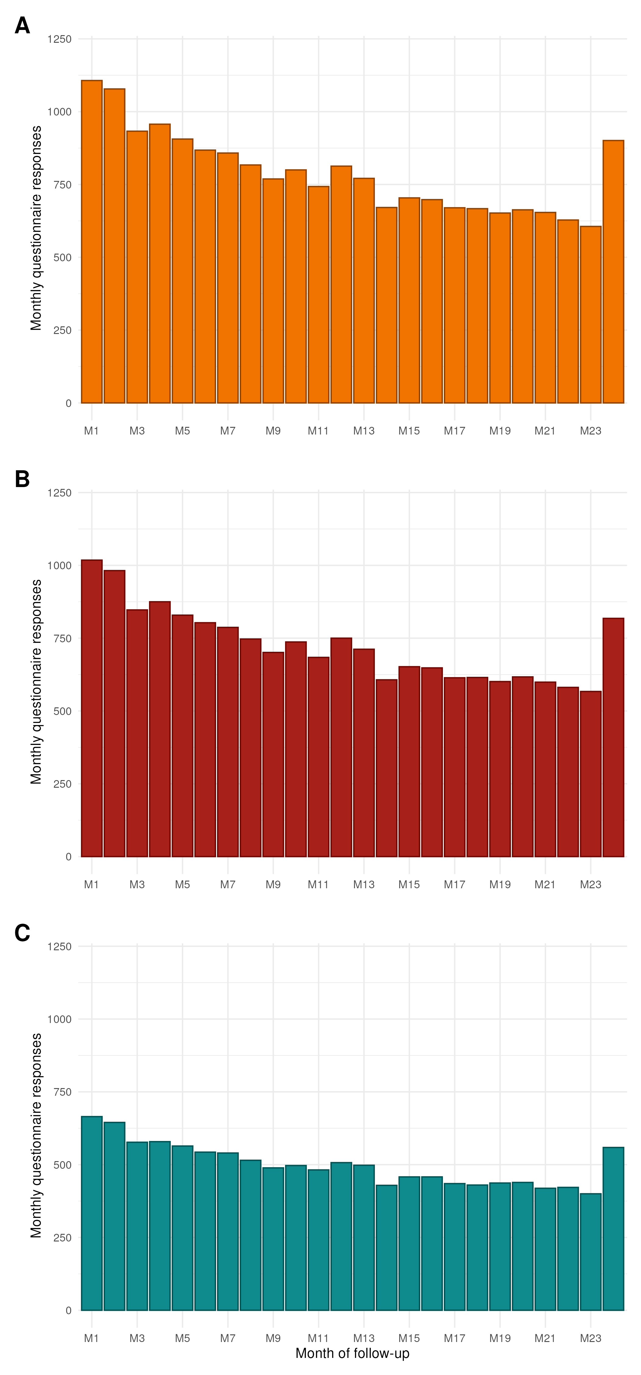
Primary outcome: First patient-reported flare
For patient-reported flares, a flare is primarily defined by a subject reporting their disease as uncontrolled. The time of the flare is given by the date the subject reported their symptoms worsening.
If a date for when the symptoms worsened is given, but the subject did not answer if their disease was uncontrolled, it is assumed their disease is not controlled (in other words, it is assumed a patient-reported flare occurred).
If a subject reported their disease as being uncontrolled, but did not give a date for the worsening of their symptoms, then the earliest date given for either an IBD outpatient appointment, emergency hospital admission, call with their IBD care team, or surgery in the questionnaire response was used. If none of these dates were provided then the date of the questionnaire response was used instead.
If an objective flare occurs prior to a patient-reported flare then the patient-reported flare is assumed to occur on the same date as the objective flare.
A complete description of the steps taken to calculate patient-reported flares is outlined in the below drop-down section.
Steps for calculating patient-reported flares
- If date of flare is before date of entry to study, then delete flare date and recode diseasecontrolled as 1.
- If flare date is after the questionnaire date (I.E in the future), reset flare date to questionnaire date.
- If questionnaire completed after date of withdrawal, remove.
- If date of flare is >2 years after entry, censor patient-reported flare at 2 years.
- Time is earliest of flare time or end of follow up, from entry date.
- All data censored at 2 years.
- Including the objective flares (objective flare data are much more straightforward, flare=
diseaseflareynand flare date=firstflarestartdatefrom EOS data)- If both datasets say no flare, patient-reported flare is no and follow up time from objective flare <= 2 years, patient-reported flare time is longest of questionnaire and objective flare times
- If both datasets say no flare, patient-reported flare is no and follow up time from objective flare > 2 years, patient-reported time is 2 years
- If no flare in questionnaires, but objective flare reported before 2 years of follow up, take objective flare data
- If no flare in questionnaires, but objective flare reported after 2 years, patient-reported flare is no and patient-reported flare time is 2 years
- If flare in questionnaire and no objective flare, patient-reported flare from questionnaire data
- If flare in questionnaire and also objective flare, take the earliest time
- If questionnaire data is missing and no objective flare, patient-reported flare is no and time is earliest of objective flare follow up and 2 years
- If questionnaire data is missing and objective flare reported within 2 years, patient-reported flare data are taken from objective flare data
- If questionnaire data is missing and objective flare reported after 2 years then patient-reported flare is no and time is 2 years
- Otherwise if questionnaire data is not missing and hardflare is, then patient-reported flare is taken from questionnaire data
All times are taken from the earliest reported flare.
Code
flare_data <- flare.df %>% drop_na(cat)
p <- create_km_flare_plot(
  data = flare_data,
  formula = Surv(softflare_time, softflare) ~ diagnosis2,
  legend_title = "IBD type",
  legend_labs = c("Crohn's disease", "UC/IBDU"),
  palette = c("#4F6D7A", "#02C3BD"),
  xlab = "Time from study recruitment (days)",
  save_path = paste0(paths$outdir, "flare-soft")
)
# Save plot to PNG for display
png("plots/flare-soft.png", width = 7, height = 7, units = "in", res = 300)
print(p, newpage = FALSE)
dev.off()
png
2 Code
knitr::include_graphics("plots/flare-soft.png")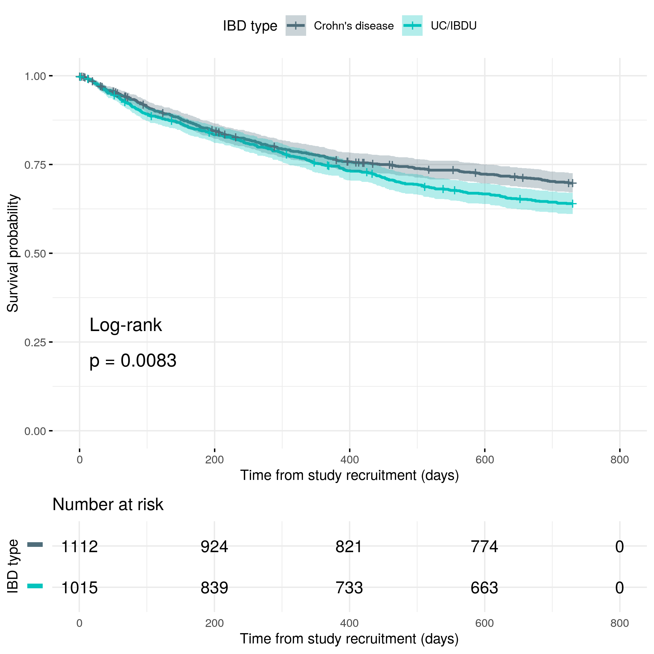
Secondary outcome: first objective flare
For the secondary outcome, disease flares have been reported by clinical care teams instead of being reported by subjects themselves.
Code
flare.df.cutoff <- flare.df %>%
mutate(
hardflare = if_else(hardflare_time > 730.5, 0, hardflare),
hardflare_time = if_else(hardflare_time > 730.5, 730.5, hardflare_time)
)
p <- create_km_flare_plot(
data = flare.df.cutoff,
formula = Surv(hardflare_time, hardflare) ~ diagnosis2,
legend_title = "IBD type",
legend_labs = c("Crohn's disease", "UC/IBDU"),
palette = c("#4F6D7A", "#02C3BD"),
xlab = "Time from study recruitment (days)"
)
# Save plot to PNG for display
png("plots/flare-hard-cutoff.png", width = 7, height = 7, units = "in", res = 300)
print(p, newpage = FALSE)
dev.off()png
2 Code
knitr::include_graphics("plots/flare-hard-cutoff.png")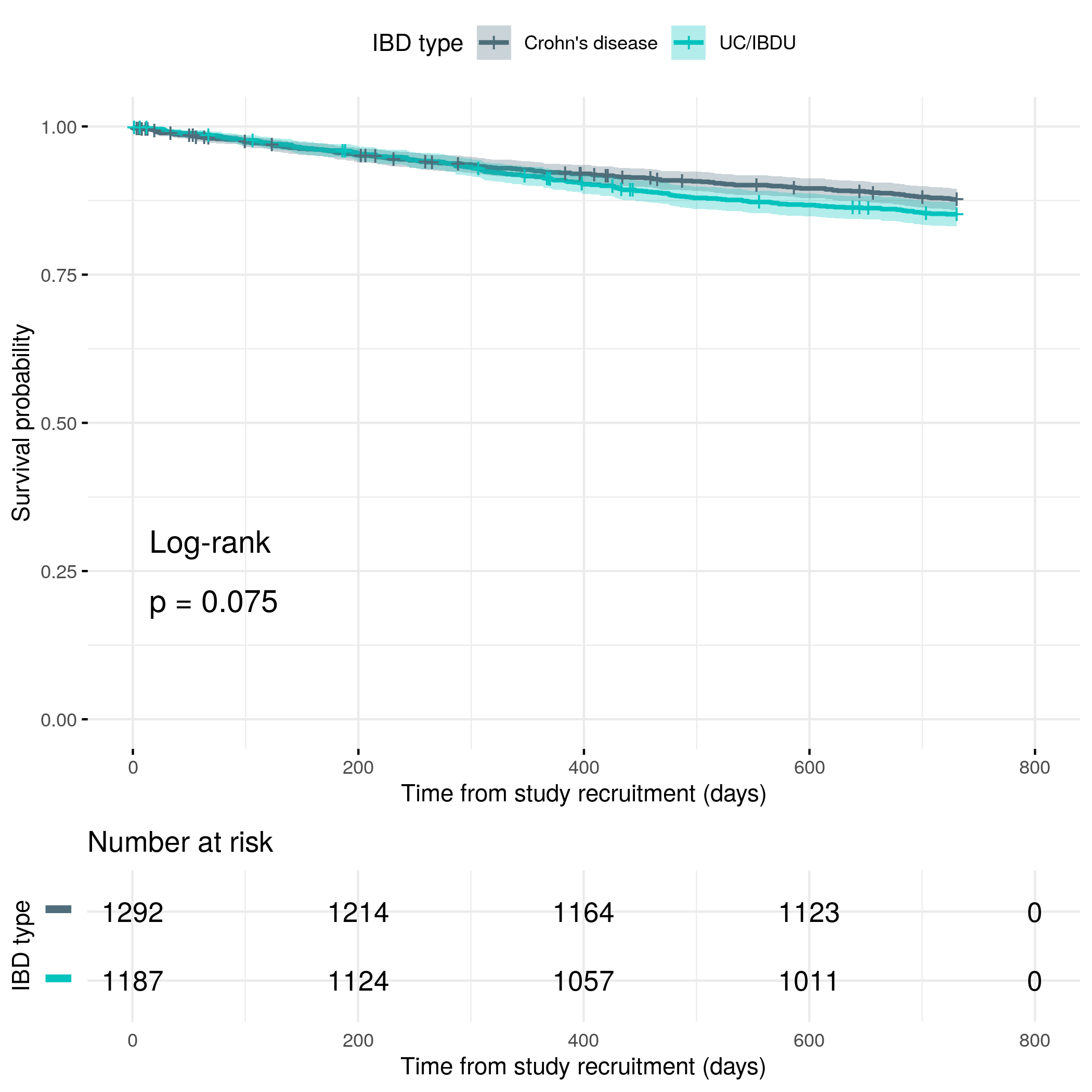
Code
fit <- survfit(Surv(hardflare_time, hardflare) ~ 1, data = flare.df)
p <- ggsurvplot(fit,
data = flare.df,
conf.int = TRUE,
pval = TRUE,
pval.method = TRUE,
ggtheme = theme_minimal(),
risk.table = TRUE,
palette = c("#4F6D7A", "#02C3BD"),
xlab = "Time from study recrutiment (days)",
break.time.by = 400
)Warning in .pvalue(fit, data = data, method = method, pval = pval, pval.coord = pval.coord, : There are no survival curves to be compared.
This is a null model.Code
fit %>%
tbl_survfit(
times = max(flare.df$hardflare_time, na.rm = TRUE),
statistic = "{estimate} ({conf.low}, {conf.high})",
label_header = "**Survival across full follow-up (95% CI)**"
)| Characteristic | Survival across full follow-up (95% CI) |
|---|---|
| Overall | 70% (67%, 74%) |
Code
p <- create_km_flare_plot(
data = flare.df,
formula = Surv(hardflare_time, hardflare) ~ diagnosis2,
legend_title = "IBD type",
legend_labs = c("Crohn's disease", "UC/IBDU"),
palette = c("#4F6D7A", "#02C3BD"),
xlab = "Time from study recruitment (days)",
save_path = paste0(paths$outdir, "flare-hard")
)
# Save plot to PNG for display
png("plots/flare-hard-diag.png", width = 7, height = 7, units = "in", res = 300)
print(p, newpage = FALSE)
dev.off()png
2 Code
knitr::include_graphics("plots/flare-hard-diag.png")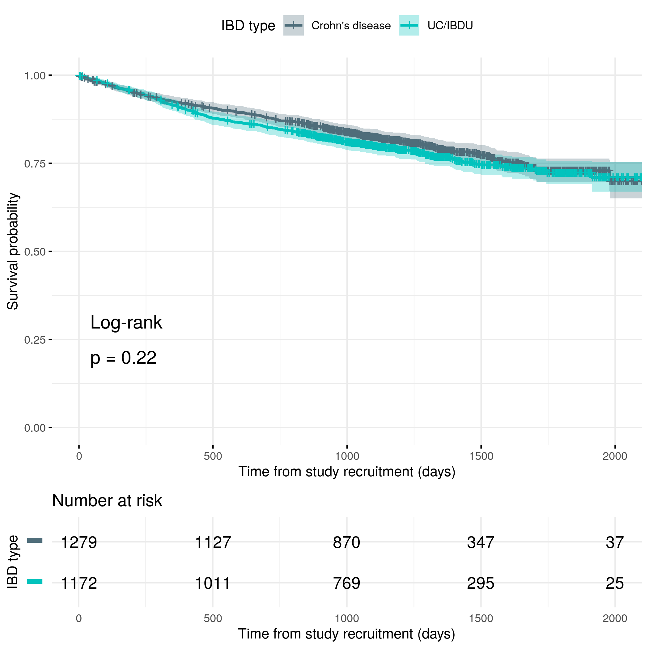
Code
fit %>%
tbl_survfit(
times = max(flare.df$hardflare_time, na.rm = TRUE),
label = "IBD type",
statistic = "{estimate} ({conf.low}, {conf.high})",
label_header = "**Survival across full follow-up (95% CI)**"
)| Characteristic | Survival across full follow-up (95% CI) |
|---|---|
| IBD type | 70% (67%, 74%) |
Comparison of hard and patient-reported flares
Code
flare.comb <- rbind(
data.frame(
ParticipantNo = flares$ParticipantNo,
Cens = flares$hardflare,
time = flares$hardflare_time,
type = "Objective flare"
),
data.frame(
ParticipantNo = flares$ParticipantNo,
Cens = flares$softflare,
time = flares$softflare_time,
type = "Patient-reported flare"
)
)
flare.comb <- flare.comb %>%
drop_na(Cens, time)
flare.comb$type <- factor(flare.comb$type,
levels = c("Objective flare", "Patient-reported flare")
)
p <- create_km_flare_plot(
data = flare.comb,
formula = Surv(time, Cens) ~ type,
legend_title = "Flare type",
legend_labs = c("Objective flare", "Patient-reported flare"),
palette = c("#DD6E42", "#EE1B65"),
xlab = "Time from study recruitment (days)",
show_pval = FALSE,
xlim = c(0, 2200),
save_path = paste0(paths$outdir, "flare-comparison")
)Scale for x is already present.
Adding another scale for x, which will replace the existing scale.Code
png
  2
Code
knitr::include_graphics("plots/flare-comparison.png")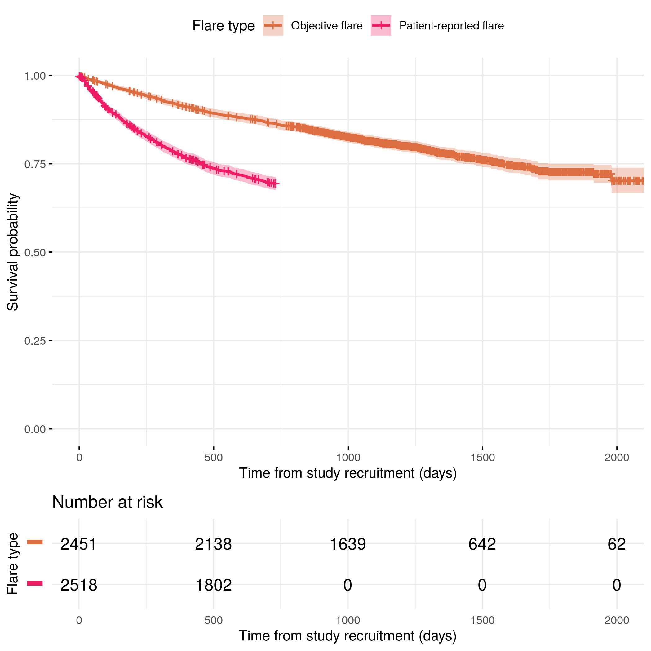
Code
fit %>%
  tbl_survfit(
    times = 365 * 1,
    label = "Flare type",
    statistic = "{estimate} ({conf.low}, {conf.high})",
    label_header = "**1-year survival (95% CI)**"
  )
fit %>%
  tbl_survfit(
    times = 365 * 2,
    label = "Flare type",
    statistic = "{estimate} ({conf.low}, {conf.high})",
    label_header = "**2-year survival (95% CI)**"
  )
fit %>%
  tbl_survfit(
    times = 365 * 3,
    label = "Flare type",
    statistic = "{estimate} ({conf.low}, {conf.high})",
    label_header = "**3-year survival (95% CI)**"
  )
fit %>%
  tbl_survfit(
    times = 365.25 * 4,
    label = "Flare type",
    statistic = "{estimate} ({conf.low}, {conf.high})",
    label_header = "**4-year survival (95% CI)**"
)| Characteristic | 1-year survival (95% CI) |
|---|---|
| Flare type | 92% (91%, 93%) |
| Characteristic | 2-year survival (95% CI) |
|---|---|
| Flare type | 86% (85%, 88%) |
| Characteristic | 3-year survival (95% CI) |
|---|---|
| Flare type | 81% (80%, 83%) |
| Characteristic | 4-year survival (95% CI) |
|---|---|
| Flare type | 77% (75%, 79%) |
Code
flare.comb.cd <- flare.comb %>%
  merge(demo[, c("ParticipantNo", "diagnosis2")], by = "ParticipantNo") %>%
  filter(diagnosis2 == "CD") %>%
  select(-diagnosis2)

fit.cd <- survfit(Surv(time, Cens) ~ type, data = flare.comb.cd)

fit.cd %>%
  tbl_survfit(
    times = 365 * 2,
    label = "Flare type",
    statistic = "{estimate} ({conf.low}, {conf.high})",
    label_header = "**2-year survival (95% CI)**"
)| Characteristic | 2-year survival (95% CI) |
|---|---|
| Flare type | |
| Objective flare | 88% (86%, 89%) |
| Patient-reported flare | 72% (69%, 74%) |
Code
flare.comb.uc <- flare.comb %>%
  merge(demo[, c("ParticipantNo", "diagnosis2")], by = "ParticipantNo") %>%
  filter(diagnosis2 == "UC/IBDU") %>%
  select(-diagnosis2)

fit.uc <- survfit(Surv(time, Cens) ~ type, data = flare.comb.uc)

fit.uc %>%
  tbl_survfit(
    times = 365 * 2,
    label = "Flare type",
    statistic = "{estimate} ({conf.low}, {conf.high})",
    label_header = "**2-year survival (95% CI)**"
)| Characteristic | 2-year survival (95% CI) |
|---|---|
| Flare type | |
| Objective flare | 85% (83%, 87%) |
| Patient-reported flare | 67% (64%, 70%) |
Reproduction and reproducibility
Session info
R version 4.4.0 (2024-04-24)
Platform: aarch64-unknown-linux-gnu
locale: LC_CTYPE=en_US.UTF-8, LC_NUMERIC=C, LC_TIME=en_US.UTF-8, LC_COLLATE=en_US.UTF-8, LC_MONETARY=en_US.UTF-8, LC_MESSAGES=en_US.UTF-8, LC_PAPER=en_US.UTF-8, LC_NAME=C, LC_ADDRESS=C, LC_TELEPHONE=C, LC_MEASUREMENT=en_US.UTF-8 and LC_IDENTIFICATION=C
attached base packages: stats, graphics, grDevices, utils, datasets, methods and base
other attached packages: gtsummary(v.1.7.2), DescTools(v.0.99.54), finalfit(v.1.0.7), coxme(v.2.2-20), bdsmatrix(v.1.3-7), pander(v.0.6.5), survminer(v.0.4.9), ggpubr(v.0.6.0), survival(v.3.5-8), datefixR(v.1.6.1), lubridate(v.1.9.3), forcats(v.1.0.0), stringr(v.1.5.1), dplyr(v.1.1.4), purrr(v.1.0.2), readr(v.2.1.5), tidyr(v.1.3.1), tibble(v.3.2.1), ggplot2(v.3.5.1), tidyverse(v.2.0.0), readxl(v.1.4.3) and patchwork(v.1.2.0)
loaded via a namespace (and not attached): gridExtra(v.2.3), gld(v.2.6.6), rlang(v.1.1.3), magrittr(v.2.0.3), e1071(v.1.7-14), compiler(v.4.4.0), systemfonts(v.1.3.1), vctrs(v.0.6.5), pkgconfig(v.2.0.3), shape(v.1.4.6.1), fastmap(v.1.2.0), backports(v.1.5.0), labeling(v.0.4.3), KMsurv(v.0.1-5), utf8(v.1.2.4), rmarkdown(v.2.27), markdown(v.1.12), tzdb(v.0.4.0), nloptr(v.2.0.3), ragg(v.1.3.2), xfun(v.0.44), glmnet(v.4.1-8), jomo(v.2.7-6), jsonlite(v.1.8.8), pan(v.1.9), broom(v.1.0.6), R6(v.2.5.1), stringi(v.1.8.4), car(v.3.1-2), boot(v.1.3-30), rpart(v.4.1.23), cellranger(v.1.1.0), Rcpp(v.1.0.12), iterators(v.1.0.14), knitr(v.1.47), zoo(v.1.8-12), Matrix(v.1.7-0), splines(v.4.4.0), nnet(v.7.3-19), timechange(v.0.3.0), tidyselect(v.1.2.1), rstudioapi(v.0.16.0), abind(v.1.4-5), yaml(v.2.3.8), ggtext(v.0.1.2), codetools(v.0.2-20), lattice(v.0.22-6), withr(v.3.0.0), evaluate(v.0.23), proxy(v.0.4-27), xml2(v.1.3.6), survMisc(v.0.5.6), pillar(v.1.9.0), carData(v.3.0-5), mice(v.3.16.0), foreach(v.1.5.2), generics(v.0.1.3), hms(v.1.1.3), commonmark(v.1.9.1), munsell(v.0.5.1), scales(v.1.3.0), rootSolve(v.1.8.2.4), minqa(v.1.2.7), xtable(v.1.8-4), class(v.7.3-22), glue(v.1.7.0), lmom(v.3.0), tools(v.4.4.0), data.table(v.1.15.4), lme4(v.1.1-35.3), ggsignif(v.0.6.4), Exact(v.3.2), mvtnorm(v.1.2-5), grid(v.4.4.0), colorspace(v.2.1-0), nlme(v.3.1-164), cli(v.3.6.2), km.ci(v.0.5-6), textshaping(v.0.4.0), fansi(v.1.0.6), expm(v.0.999-9), broom.helpers(v.1.15.0), gt(v.0.10.1), gtable(v.0.3.5), rstatix(v.0.7.2), sass(v.0.4.9), digest(v.0.6.35), farver(v.2.1.2), htmlwidgets(v.1.6.4), htmltools(v.0.5.8.1), lifecycle(v.1.0.4), httr(v.1.4.7), mitml(v.0.4-5), gridtext(v.0.1.5) and MASS(v.7.3-60.2)
Licensed by CC BY unless otherwise stated.