Diet

Nathan Constantine-Cooke; Beatriz Gros; Maiara Brusco De Freitas

Diet

Authors

Affiliations

Nathan Constantine-Cooke

Institute of Genetics and Cancer

Beatriz Gros

Reina Sofía University Hospital, Gastroenterology and Hepatology

Edinburgh IBD Unit

Maiara Brusco De Freitas

Center for Molecular Prediction of Inflammatory Bowel Disease (PREDICT), Aalborg University

Published

January 13, 2026

Introduction

Code

set.seed(123)

source("Baseline/utils.R")

##############
## Packages ##
##############

library(plyr) # Used for mapping values
suppressPackageStartupMessages(library(tidyverse)) # ggplot2, dplyr, and magrittr
library(readxl) # Read in Excel files
library(lubridate) # Handle dates
library(datefixR) # Standardise dates
library(patchwork) # Arrange ggplots

# Generate tables
suppressPackageStartupMessages(library(table1))
library(knitr)
library(pander)

# Generate flowchart of cohort derivation
library(DiagrammeR)
library(DiagrammeRsvg)

# paths to PREdiCCt data
if (file.exists("/docker")) { # If running in docker
  data.path <- "data/final/20221004/"
  redcap.path <- "data/final/20231030/"
  upf.path <- "data/final/20240924/"
  prefix <- "data/end-of-follow-up/"
  outdir <- "data/processed/"
} else { # Run on OS directly
  data.path <- "/Volumes/igmm/cvallejo-predicct/predicct/final/20221004/"
  redcap.path <- "/Volumes/igmm/cvallejo-predicct/predicct/final/20231030/"
  upf.path <- "/Volumes/igmm/cvallejo-predicct/predicct/final/20240924/"
  prefix <- "/Volumes/igmm/cvallejo-predicct/predicct/end-of-follow-up/"
  outdir <- "/Volumes/igmm/cvallejo-predicct/predicct/processed/"
}

demo <- readRDS(paste0(outdir, "demo-biochem.RDS"))

FFQ <- read_xlsx(paste0(
  prefix,
  "predicct ffq_nutrientfood groupDQI all foods_data (n1092)Nov2022.xlsx"
))

FFQ$meat_overall <- rowSums(FFQ[, paste0("meat7", letters[1:12], "_grams")])

FFQ$fish_overall <- rowSums(FFQ[, paste0("fish8", letters[1:13], "_grams")])

FFQ$ParticipantNo <- FFQ$participantno
demo <- merge(demo,
  FFQ[, c(
    "ParticipantNo",
    "Meat_sum",
    "meat_overall",
    "fish_overall",
    "fibre",
    "PUFA_percEng",
    "NOVAScore_cat",
    "dqi_tot"
  )],
  by = "ParticipantNo",
  all.x = TRUE,
  all.y = FALSE
)

cat_theme <- function(gg) {
  p <- gg +
    scale_fill_manual(values = c("#DA4167", "#F4D35E", "#083D77")) +
    scale_color_manual(values = colorspace::darken(c("#DA4167",
                                                     "#F4D35E",
                                                     "#083D77"),
                                                   0.2)
                     ) +
  theme_minimal()
  p
}

PREdiCCt has collected data on diet via food frequency questionnaires (FFQs) and food diaries. This dietary data has been analysed by staff at the University of Aberdeen, primarily by Dr Janet Kyle, Dr Graham Horgan, and Professor Alex Johnstone.

Whilst data for many dietary variables have been collected, this report will focus on the data outlined in the SAP.

Protein from animal-sources
Dietary fibre
Polyunsaturated fatty acids (PUFAs)
Nova intake score

The data for these variables were extracted from the FFQs. As reported associations between dietary data and IBD are often specific to a form of IBD rather than IBD as a whole, these data will be presented stratified by disease type.

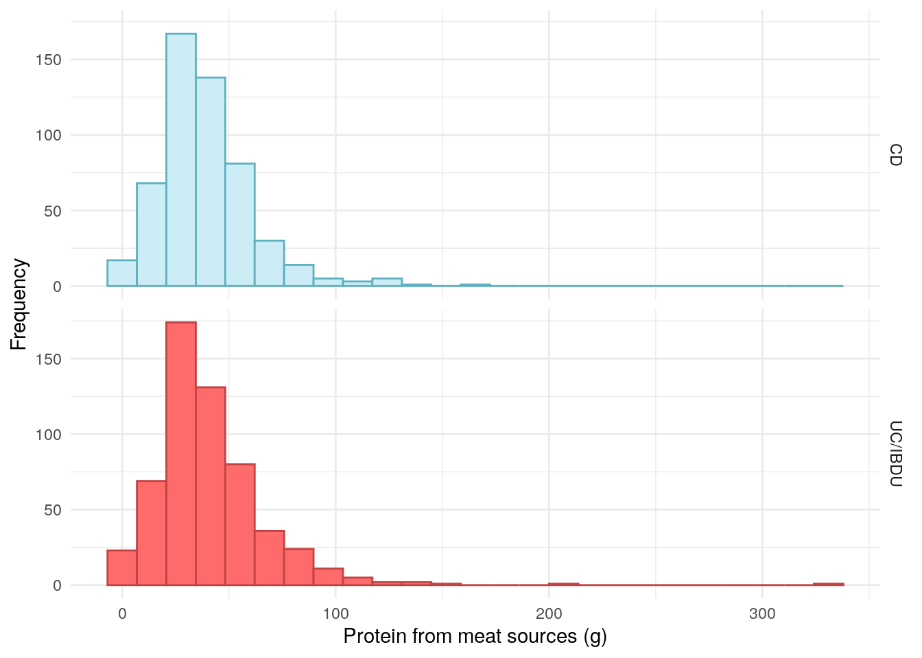
Protein from meat sources

Figure 1 suggests there are relatively few vegetarians in the PREdiCCt cohort. Whilst some extreme values were observed for protein from meat sources, they remain plausible.

Code

demo %>%
  drop_na(Meat_sum) %>%
  ggplot(aes(x = Meat_sum, color = diagnosis2, fill = diagnosis2)) +
  geom_histogram(bins = 25) +
  theme_minimal() +
  theme(legend.position = "none") +
  labs(
    x = "Protein from meat sources (g)",
    y = "Frequency",
    color = "IBD type",
    fill = "IBD type"
  ) +
  scale_fill_manual(
    labels = c("UC/IBDU", "Crohn's"),
    values = c("#CDEDF6", "#FF6B6B")
  ) +
  scale_color_manual(
    labels = c("UC/IBDU", "Crohn's"),
    values = c("#5EB1BF", "#C24343")
  ) +
  facet_grid(rows = vars(diagnosis2))

Figure 1: Distribution of protein intake from meat.

No association was observed between protein intake from meat and FC in either CD or UC.

Code

demo %>%
  filter(diagnosis2 == "CD") %>%
  aov(formula = Meat_sum ~ cat) %>%
  summary() %>%
  pander()

Table 1: ANOVA between protein intake from meat and FC groups in Crohn’s disease.

Analysis of Variance Model
	Df	Sum Sq	Mean Sq	F value	Pr(>F)
cat	2	237.6	118.8	0.2419	0.7852
Residuals	494	242579	491.1	NA	NA

Code

demo %>%
  filter(diagnosis2 == "UC/IBDU") %>%
  aov(formula = Meat_sum ~ cat) %>%
  summary() %>%
  pander()

Table 2: ANOVA between protein intake from meat and FC groups in UC/IBDU.

Analysis of Variance Model
	Df	Sum Sq	Mean Sq	F value	Pr(>F)
cat	2	3350	1675	2.814	0.06088
Residuals	512	304730	595.2	NA	NA

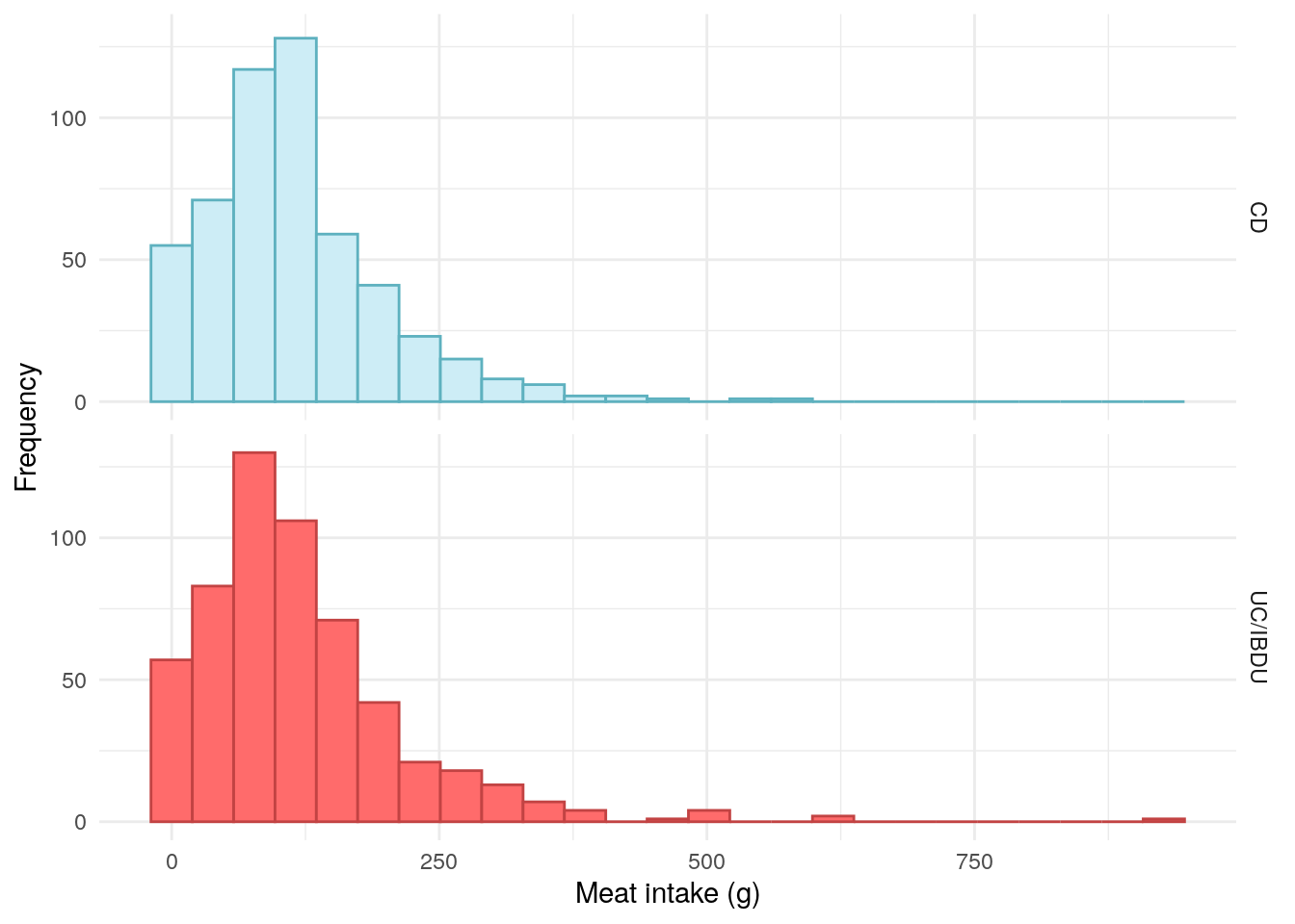
Overall meat intake

Code

demo %>%
  drop_na(meat_overall) %>%
  ggplot(aes(x = meat_overall, color = diagnosis2, fill = diagnosis2)) +
  geom_histogram(bins = 25) +
  theme_minimal() +
  theme(legend.position = "none") +
  labs(
    x = "Meat intake (g)",
    y = "Frequency",
    color = "IBD type",
    fill = "IBD type"
  ) +
  scale_fill_manual(
    labels = c("UC/IBDU", "Crohn's"),
    values = c("#CDEDF6", "#FF6B6B")
  ) +
  scale_color_manual(
    labels = c("UC/IBDU", "Crohn's"),
    values = c("#5EB1BF", "#C24343")
  ) +
  facet_grid(rows = vars(diagnosis2))

Figure 2: Distribution of overall meat intake.

No association was observed between meat intake and FC in CD. However, a significant association was observed between meat intake and FC in UC/IBDU Table 4.

Code

demo %>%
  filter(diagnosis2 == "CD") %>%
  aov(formula = meat_overall ~ cat) %>%
  summary() %>%
  pander()

Table 3: ANOVA between meat intake and FC groups in Crohn’s disease.

Analysis of Variance Model
	Df	Sum Sq	Mean Sq	F value	Pr(>F)
cat	2	730.4	365.2	0.05301	0.9484
Residuals	494	3403211	6889	NA	NA

Code

demo %>%
  filter(diagnosis2 == "UC/IBDU") %>%
  aov(formula = meat_overall ~ cat) %>%
  summary() %>%
  pander()

Table 4: ANOVA between meat intake and FC groups in UC/IBDU.

Analysis of Variance Model
	Df	Sum Sq	Mean Sq	F value	Pr(>F)
cat	2	69131	34565	4.373	0.01309
Residuals	512	4046939	7904	NA	NA

Code

p <- demo %>%
  filter(diagnosis2 == "UC/IBDU") %>%
  drop_na(cat, meat_overall) %>%
  mutate(cat = fct_rev(cat)) %>%
  ggplot(aes(x = meat_overall, fill = cat, color = cat)) +
  geom_density() +
  facet_grid(rows = vars(cat)) +
  labs(x = "Meat intake",
       y = "Density",
       fill = "FC group",
       color = "FC group")
cat_theme(p)

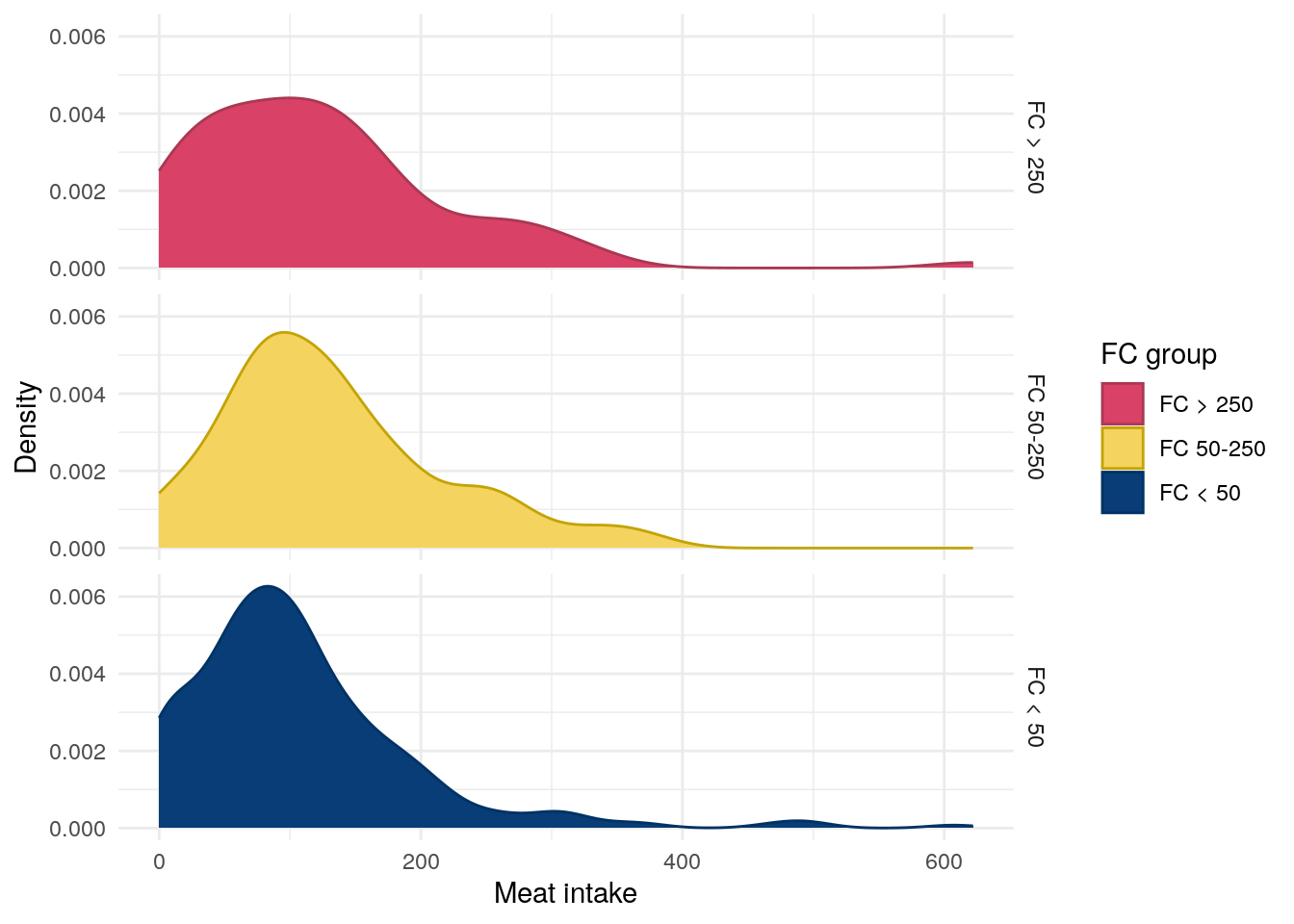
Figure 3: Distribution of meat intake by FC in UC.

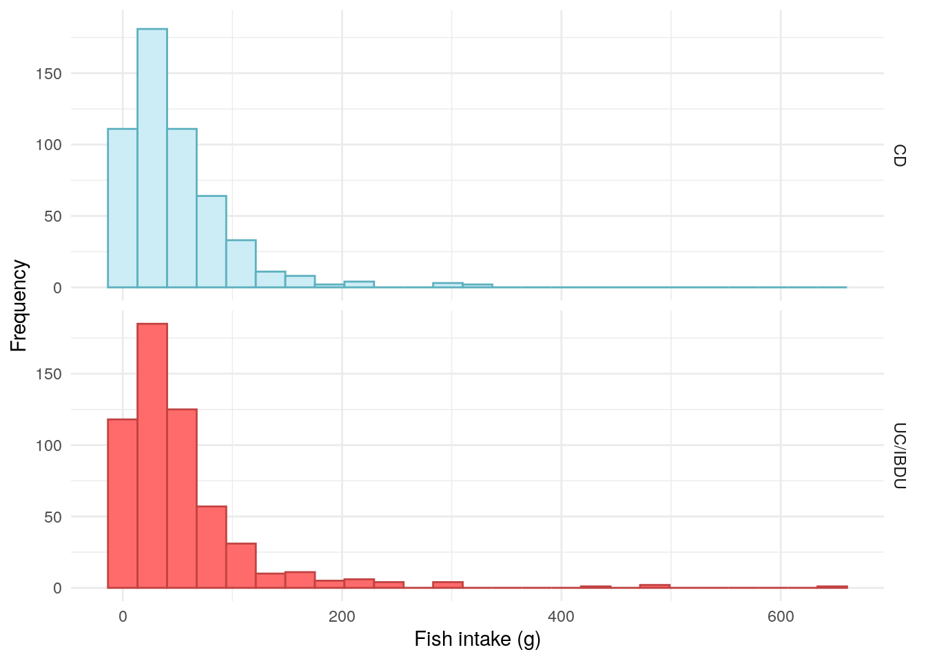
Overall fish intake

Code

demo %>%
  drop_na(fish_overall) %>%
  ggplot(aes(x = fish_overall, color = diagnosis2, fill = diagnosis2)) +
  geom_histogram(bins = 25) +
  theme_minimal() +
  theme(legend.position = "none") +
  labs(
    x = "Fish intake (g)",
    y = "Frequency",
    color = "IBD type",
    fill = "IBD type"
  ) +
  scale_fill_manual(
    labels = c("UC/IBDU", "Crohn's"),
    values = c("#CDEDF6", "#FF6B6B")
  ) +
  scale_color_manual(
    labels = c("UC/IBDU", "Crohn's"),
    values = c("#5EB1BF", "#C24343")
  ) +
  facet_grid(rows = vars(diagnosis2))

Figure 4: Distribution of overall fish intake.

No association was observed between meat intake and FC in CD. However, a significant association was observed between meat intake and FC in UC/IBDU Table 4.

Code

demo %>%
  filter(diagnosis2 == "CD") %>%
  aov(formula = fish_overall ~ cat) %>%
  summary() %>%
  pander()

Table 5: ANOVA between fish intake and FC groups in Crohn’s disease.

Analysis of Variance Model
	Df	Sum Sq	Mean Sq	F value	Pr(>F)
cat	2	4855	2427	1.085	0.3388
Residuals	494	1105599	2238	NA	NA

Code

demo %>%
  filter(diagnosis2 == "UC/IBDU") %>%
  aov(formula = fish_overall ~ cat) %>%
  summary() %>%
  pander()

Table 6: ANOVA between fish intake and FC groups in UC/IBDU.

Analysis of Variance Model
	Df	Sum Sq	Mean Sq	F value	Pr(>F)
cat	2	1986	992.9	0.2838	0.753
Residuals	512	1791051	3498	NA	NA

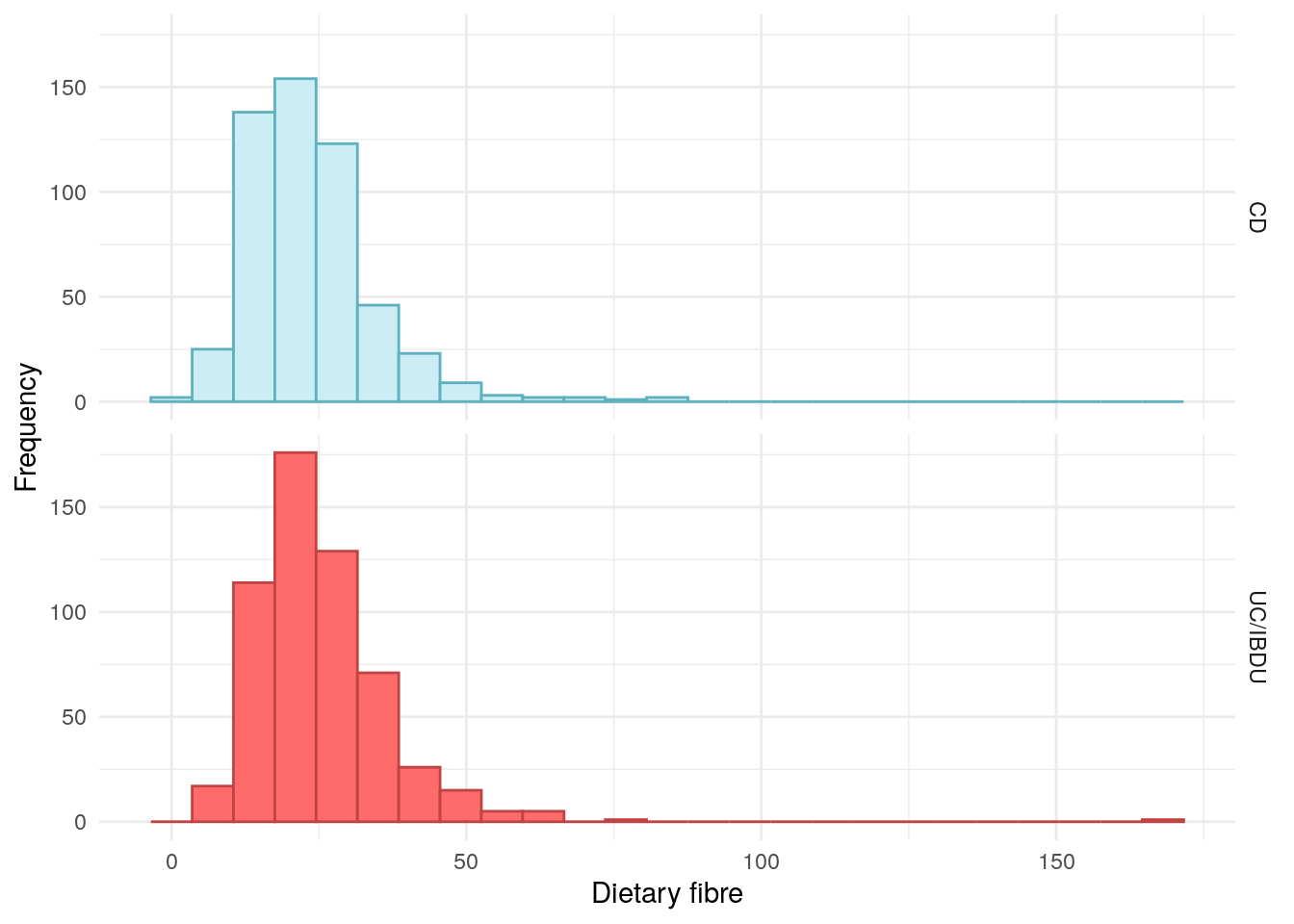
Dietary fibre

Fibre has frequently investigated as a potential factor in IBD pathogenesis, particularly in CD.

A study of 170,776 women across 26 years found fibre intake, particularly fibre derived from fruits, to be low for incident CD patients (Ananthakrishnan et al. 2013).

A US study of 1,130 CD subjects found CD patients who reported that they did not avoid high-fibre foods were approximately 40% less likely to have a disease flare in a 6-month period than those who avoided high-fibre foods (Brotherton et al. 2016).

There is less evidence of a relationship between UC and dietary fibre.

There does not appear to be substantial differences in fibre between CD and UC/IBDU PREdiCCt participants.

Code

demo %>%
  drop_na(fibre) %>%
  ggplot(aes(x = fibre, color = diagnosis2, fill = diagnosis2)) +
  geom_histogram(bins = 25) +
  theme_minimal() +
  theme(legend.position = "none") +
  labs(
    x = "Dietary fibre",
    y = "Frequency",
    color = "IBD type",
    fill = "IBD type"
  ) +
  scale_fill_manual(
    values = c("#CDEDF6", "#FF6B6B")
  ) +
  scale_color_manual(
    values = c("#5EB1BF", "#C24343")
  ) +
  facet_grid(rows = vars(diagnosis2))

Figure 5: Distribution of dietary fibre.

No association was found between dietary fibre intake and FC.

Code

demo %>%
  filter(diagnosis2 == "CD") %>%
  aov(formula = fibre ~ cat) %>%
  summary() %>%
  pander()

Table 7: ANOVA between dietary fibre and FC groups in Crohn’s disease.

Analysis of Variance Model
	Df	Sum Sq	Mean Sq	F value	Pr(>F)
cat	2	333.4	166.7	1.496	0.2251
Residuals	494	55046	111.4	NA	NA

Code

demo %>%
  filter(diagnosis2 == "UC/IBDU") %>%
  aov(formula = fibre ~ cat) %>%
  summary() %>%
  pander()

Table 8: ANOVA between dietary fibre and FC groups in UC/IBDU.

Analysis of Variance Model
	Df	Sum Sq	Mean Sq	F value	Pr(>F)
cat	2	80.2	40.1	0.3739	0.6882
Residuals	512	54910	107.2	NA	NA

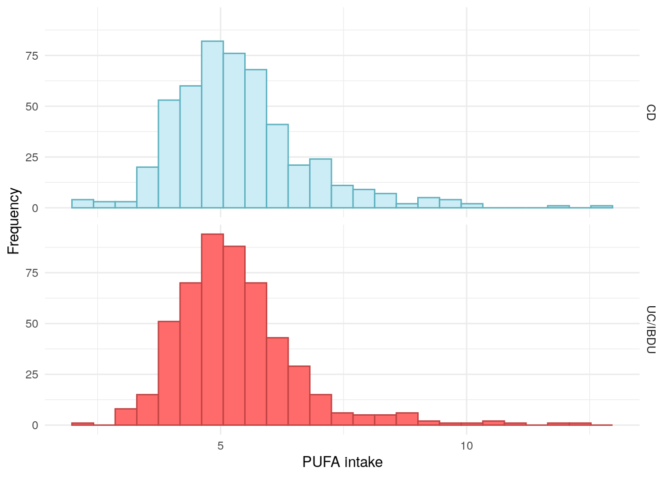
Polyunsaturated fatty acids

PUFAs exhibit anti-inflammatory properties and there is evidence of a relationship between PUFAs and UC incidence (Marion-Letellier et al. 2013). Research suggests that a diet with a poor balance of n-3 and n-6 PUFAs, commonly seen in “Western” diets is associated with IBD risk.

The PREdiCCt SAP states n-6 PUFAs will be examined. However, the data obtained from the FFQs describes PUFAs as a whole (including n-3 PUFAs).

Code

demo %>%
  drop_na(cat) %>%
  ggplot(aes(x = PUFA_percEng, color = diagnosis2, fill = diagnosis2)) +
  geom_histogram(bins = 25) +
  theme_minimal() +
  theme(legend.position = "none") +
  labs(
    x = "PUFA intake",
    y = "Frequency",
    color = "IBD type",
    fill = "IBD type"
  ) +
  scale_fill_manual(
    values = c("#CDEDF6", "#FF6B6B")
  ) +
  scale_color_manual(
    values = c("#5EB1BF", "#C24343")
  ) +
  facet_grid(rows = vars(diagnosis2))

Figure 6: Distribution of polyunsaturated fatty acids.

A significant association was not seen between PUFA intake and FC.

Code

demo %>%
  filter(diagnosis2 == "CD") %>%
  aov(formula = PUFA_percEng ~ cat) %>%
  summary() %>%
  pander()

Table 9: ANOVA between polyunsaturated fatty acids and FC groups in Crohn’s disease.

Analysis of Variance Model
	Df	Sum Sq	Mean Sq	F value	Pr(>F)
cat	2	0.9349	0.4674	0.2489	0.7798
Residuals	494	927.9	1.878	NA	NA

Code

demo %>%
  filter(diagnosis2 == "UC/IBDU") %>%
  aov(formula = PUFA_percEng ~ cat) %>%
  summary() %>%
  pander()

Table 10: ANOVA between polyunsaturated fatty acids and FC groups in UC/IBDU.

Analysis of Variance Model
	Df	Sum Sq	Mean Sq	F value	Pr(>F)
cat	2	10.72	5.359	3.378	0.03487
Residuals	512	812.1	1.586	NA	NA

Code

p <- demo %>%
  filter(diagnosis2 == "UC/IBDU") %>%
  drop_na(cat, PUFA_percEng) %>%
  mutate(cat = fct_rev(cat)) %>%
  ggplot(aes(x = PUFA_percEng, fill = cat, color = cat)) +
  geom_density() +
  facet_grid(rows = vars(cat)) +
  labs(x = "PUFA intake",
       y = "Density",
       fill = "FC group",
       color = "FC group")
cat_theme(p)

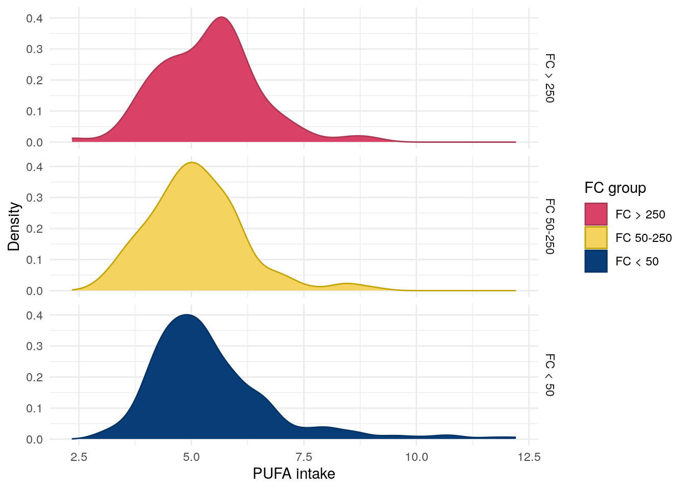
Figure 7: Distribution ofpolyunsaturated fatty acid intake by FC in UC.

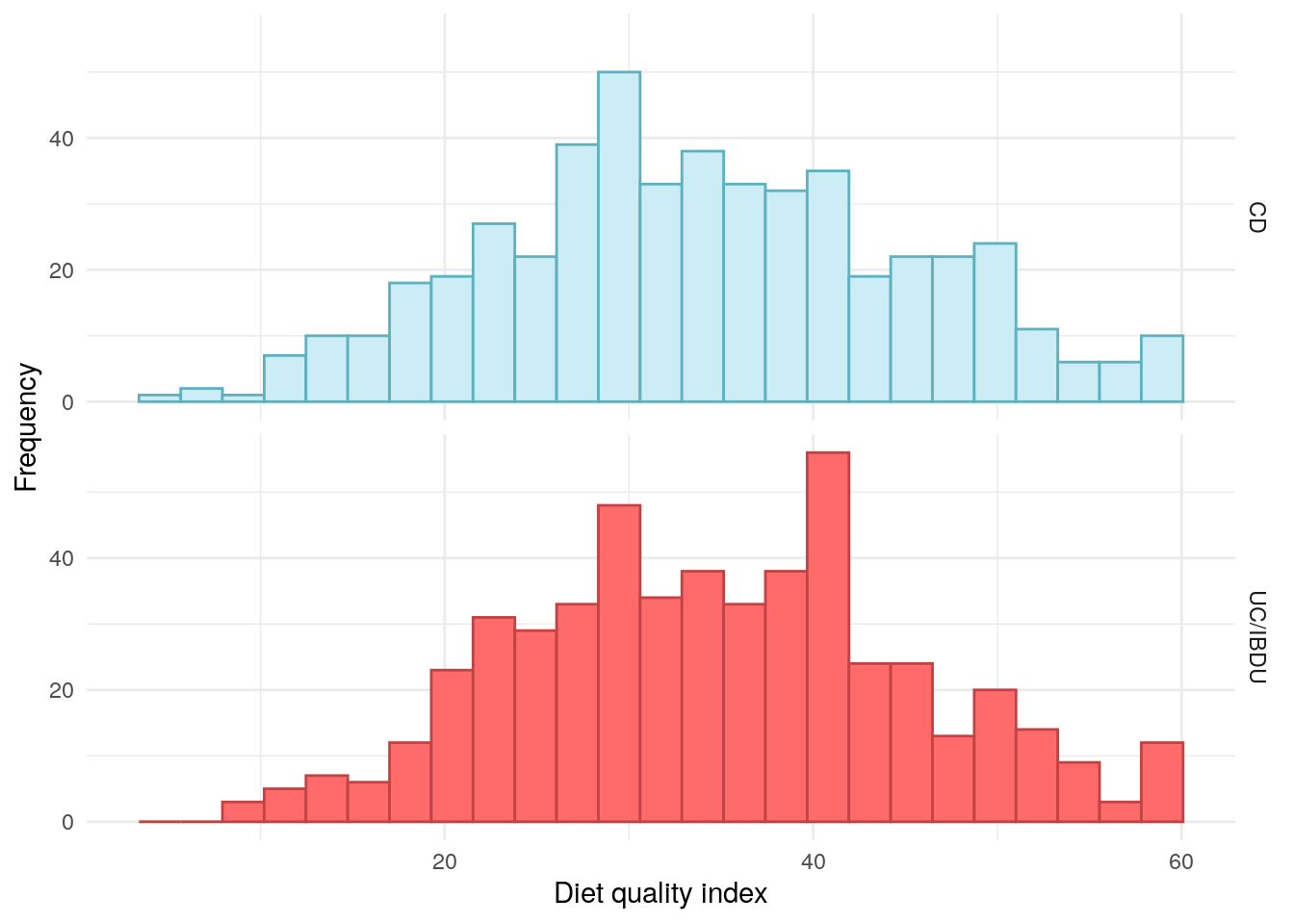
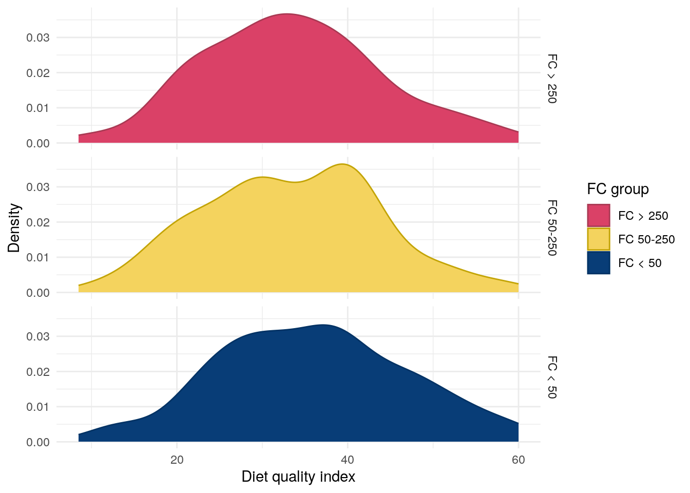
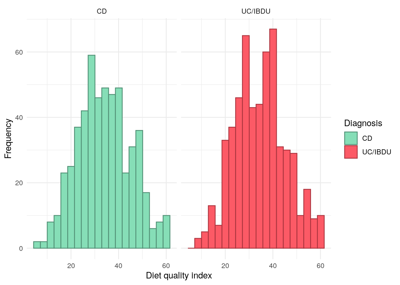
Diet qualiy index

Diet quality index (DQI) is a measure of overall diet quality ranging from 0 to 100. A higher DQI indicates a diverse diet likely meeting recommended daily intakes but reflecting moderation whilst low values indicate the converse. We used Diet Quality Index-International (DQI-I) which has been validated for use in diverse populations (Kim et al. 2003). It should be noted DQI does not necessarily relate to ultra-processed food intake.

Code

demo %>%
  drop_na(cat) %>%
  ggplot(aes(x = dqi_tot, color = diagnosis2, fill = diagnosis2)) +
  geom_histogram(bins = 25) +
  theme_minimal() +
  theme(legend.position = "none") +
  labs(
    x = "Diet quality index",
    y = "Frequency",
    color = "IBD type",
    fill = "IBD type"
  ) +
  scale_fill_manual(
    values = c("#CDEDF6", "#FF6B6B")
  ) +
  scale_color_manual(
    values = c("#5EB1BF", "#C24343")
  ) +
  facet_grid(rows = vars(diagnosis2))

Warning: Removed 1132 rows containing non-finite outside the scale range
(`stat_bin()`).

Code

demo %>%
  filter(diagnosis2 == "CD") %>%
  aov(formula = dqi_tot ~ cat) %>%
  summary() %>%
  pander()

Table 11: ANOVA between diet quality index and FC groups in Crohn’s disease.

Analysis of Variance Model
	Df	Sum Sq	Mean Sq	F value	Pr(>F)
cat	2	121.6	60.8	0.4786	0.62
Residuals	494	62761	127	NA	NA

Code

demo %>%
  filter(diagnosis2 == "UC/IBDU") %>%
  aov(formula = dqi_tot ~ cat) %>%
  summary() %>%
  pander()

Table 12: ANOVA between diet quality index and FC groups in UC/IBDU.

Analysis of Variance Model
	Df	Sum Sq	Mean Sq	F value	Pr(>F)
cat	2	769.2	384.6	3.393	0.03436
Residuals	512	58031	113.3	NA	NA

Code

p <- demo %>%
  filter(diagnosis2 == "UC/IBDU") %>%
  drop_na(cat, dqi_tot) %>%
  mutate(cat = fct_rev(cat)) %>%
  ggplot(aes(x = dqi_tot, fill = cat, color = cat)) +
  geom_density() +
  facet_grid(rows = vars(cat)) +
  labs(x = "Diet quality index",
       y = "Density",
       fill = "FC group",
       color = "FC group")
cat_theme(p)

Figure 8: Distribution of diet quality index by FC in UC.

Nova intake score

There has been a great deal of recent research interest in ultra processed food (UPF) and IBD. For example, Narula et al. (2021) found UPF intake to be positively associated with IBD risk.

The Nova score is a popular approach for classifying UPFs (Monteiro et al. 2017). Food is classified as either unprocessed, processed culinary, processed food, or ultra-processed via the Nova score. The University of Aberdeen have developed an extension of the Nova score, the Nova intake score, which can be used to categorise individuals and their diets instead of individual food items.

The following definition of the Nova intake score was written by Liam McAdie during a 5th year medical elective in which he worked on the PREdiCCt dietary data. The formulae have received minor modifications, but otherwise the definitions remain unchanged from McAdie’s work.

Definition

When completing the FFQ, participants were asked to report (a) portion size normally consumed, (b) number of times this portion is consumed in one day and (c) number of days per week food type is consumed. Participant’s daily average consumption (in grams) of a food and drink type (x) was calculated by:

x=\frac{c}{7}(a+b)

Standardised number of portions consumed daily for food and drink type (y) was calculated by dividing consumption (x) by the Foods Standard Agency average UK-portion size (z).

y= \frac{x}{z}

Nova intake scores (N) were calculated by multiplying the number of standardised portions consumed (y) by their corresponding Nova score (M) assigned in the database. This process is repeated for all 169 food and drink types and totalled to give one overall Nova intake score. This score is a marker representative of UPF intake.

N = \sum_{i = 1}^{169} (y_i M_i)

Results

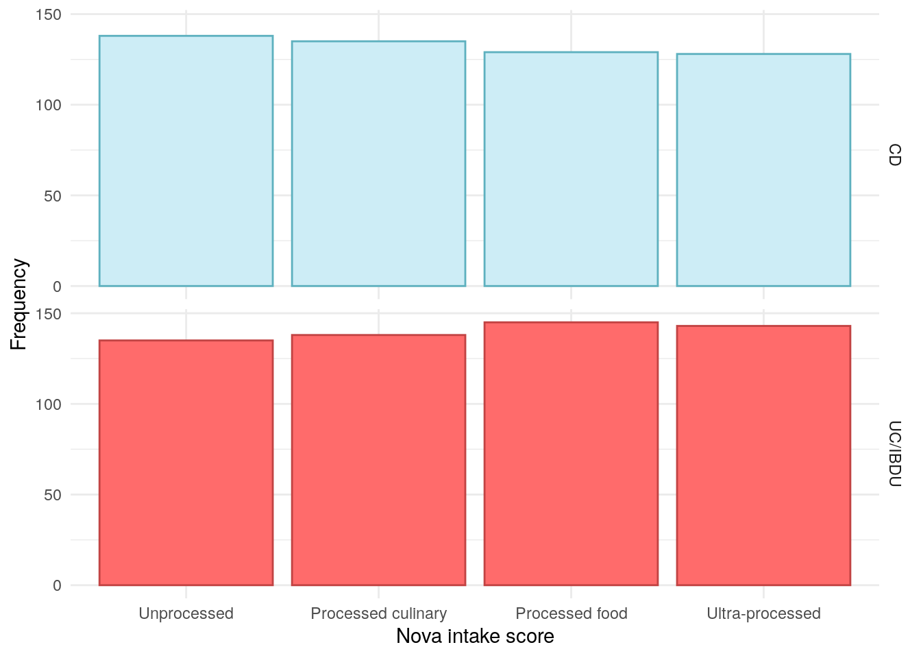
The distribution of Nova intake score appears to be uniform across the cohort, as such, it seems likely that these data have been mapped to quantiles and are no longer describing Nova Score categories.

Code

demo$NOVAScore_cat <- factor(demo$NOVAScore_cat,
  levels = 1:4,
  labels = c(
    "Unprocessed",
    "Processed culinary",
    "Processed food",
    "Ultra-processed"
  )
)

demo %>%
  drop_na(NOVAScore_cat) %>%
  ggplot(aes(x = NOVAScore_cat, color = diagnosis2, fill = diagnosis2)) +
  geom_bar() +
  theme_minimal() +
  theme(legend.position = "none") +
  labs(
    x = "Nova intake score",
    y = "Frequency",
    color = "IBD type",
    fill = "IBD type"
  ) +
  scale_fill_manual(
    values = c("#CDEDF6", "#FF6B6B")
  ) +
  scale_color_manual(
    values = c("#5EB1BF", "#C24343")
  ) +
  facet_grid(rows = vars(diagnosis2))

Figure 9: Distribution of Nova intake scores.

No significant association was observed between Nova intake scores and FC groups.

Code

temp <- demo %>%
  filter(diagnosis2 == "CD")

pander(chisq.test(temp$NOVAScore_cat, temp$cat))

Chi-squared test between Nova intake score and FC groups in Crohn’s disease.
Test statistic	df	P value
11.12	6	0.08488

Code

temp <- demo %>%
  filter(diagnosis2 == "UC/IBDU")

pander(chisq.test(temp$NOVAScore_cat, temp$cat))

Chi-squared test between Nova intake score and FC groups in UC/IBDU.
Test statistic	df	P value
4.197	6	0.6501

Processed food subgroups

In addition to exploring UPF intake as a whole, we also explore UPF intake by subcategories. This approach is based on the methodology used by Cordova et al. (2023). The following categories have been identified by Dr Maiara Brusco De Freitas using FFQ groupings.

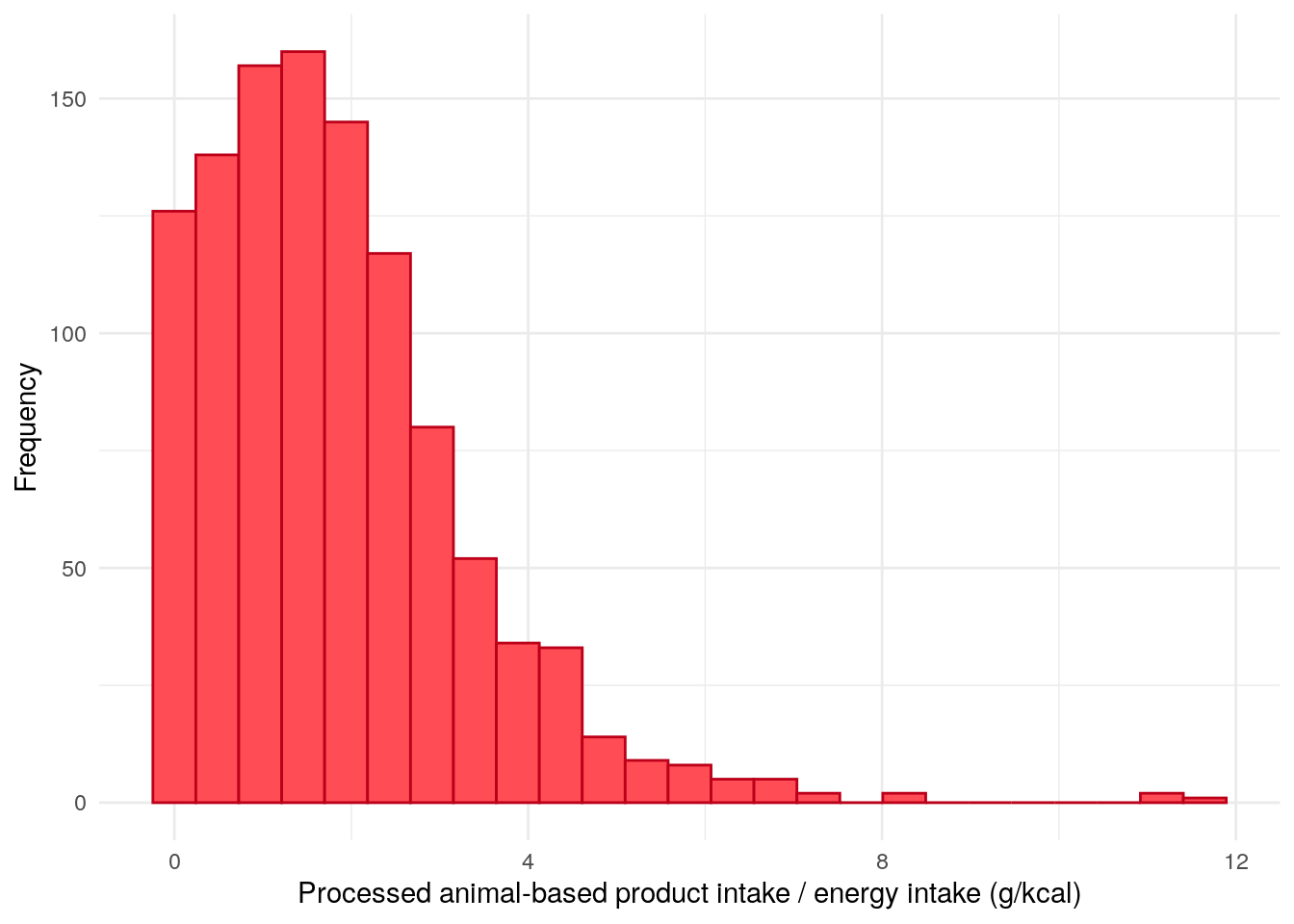
Animal-based products (processed meat) is the only subgroup considered which we found to be significantly associated with FC.

Code

FFQ$breadIntake <- with(FFQ,
                        (bread1a_grams +
                          bread1b_grams +
                          bread1c_grams +
                          bread1d_grams +
                          cereal2a_grams +
                          cereal2b_grams +
                          cereal2c_grams +
                          cereal2d_grams + 
                          cereal2e_grams) /
                          EnergykCAL) * 100

demo <- merge(demo,
              FFQ[, c("ParticipantNo", "breadIntake")],
              by = "ParticipantNo",
              all.x = TRUE,
              all.y = FALSE)

demo %>%
  drop_na(breadIntake) %>%
  ggplot(aes(x = breadIntake)) +
  geom_histogram(bins = 25, color = "#5C738F", fill = "#759EB8") +
  theme_minimal() +
  xlab("Processed bread and cereal intake / energy intake (g/kcal)") +
  ylab("Frequency")

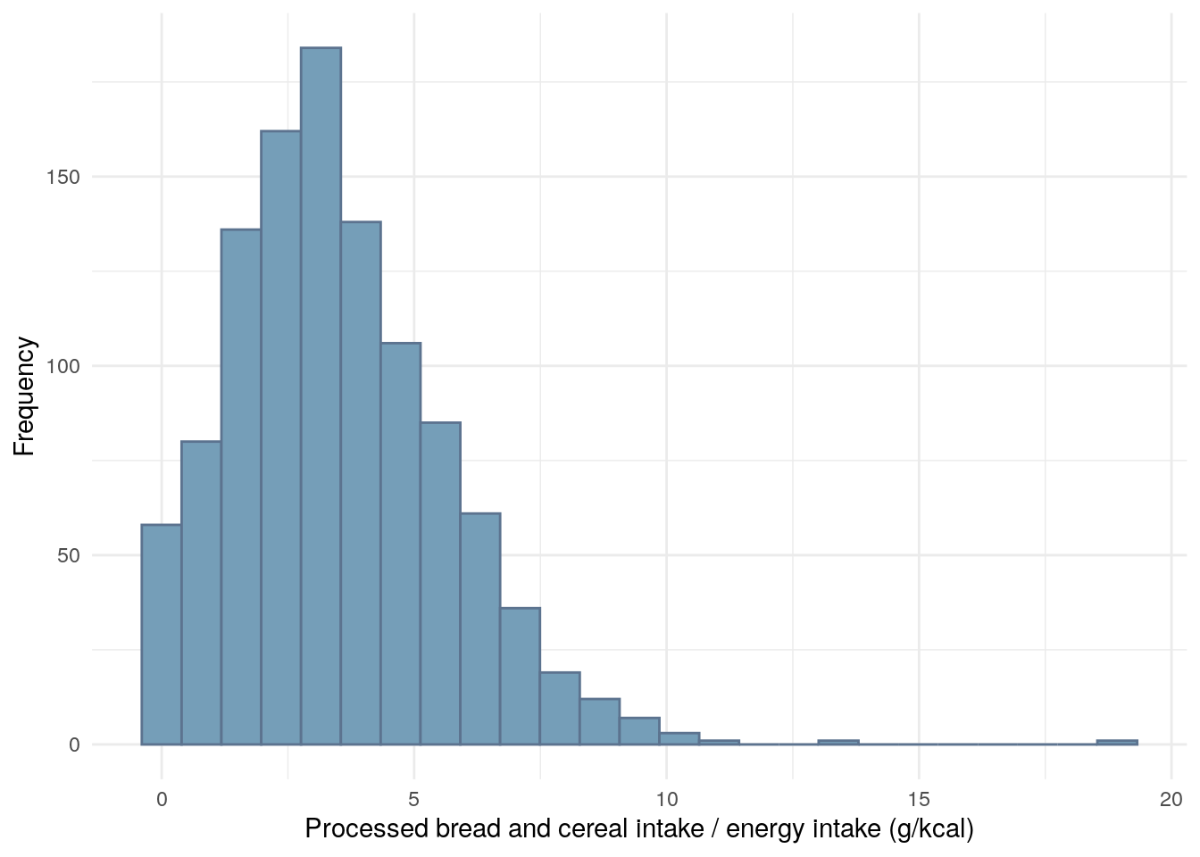
Figure 10: Distribution of processed bread and cereal intake divided by daily energy intake.

Code

pander(summary(aov(breadIntake ~ cat, data = demo)))

Table 13: ANOVA between processed bread/cereal intake and FC groups.

Analysis of Variance Model
	Df	Sum Sq	Mean Sq	F value	Pr(>F)
cat	2	15.73	7.867	1.718	0.1799
Residuals	1009	4620	4.579	NA	NA

Code

FFQ$sweetIntake <- with(FFQ,
                        (Puddings13a_grams +
                          Puddings13b_grams +
                          Puddings13c_grams +
                          Puddings13d_grams +
                          Puddings13e_grams +
                          Puddings13f_grams + 
                          Puddings13g_grams +
                          Puddings13h_grams +
                          Chocsetc14a_grams +
                          Chocsetc14b_grams +
                          Chocsetc14c_grams +
                          Chocsetc14d_grams +
                          Chocsetc14g_grams +
                          Chocsetc14h_grams +
                          Chocsetc14i_grams +
                          Biscuits15a_grams +
                          Biscuits15b_grams +
                          Biscuits15c_grams +
                          Biscuits15d_grams +
                          Biscuits15e_grams +
                          Biscuits15g_grams +
                          Cakes16a_grams +
                          Cakes16b_grams +
                          Cakes16c_grams +
                          Cakes16d_grams +
                          Cakes16e_grams) /
                          EnergykCAL) * 100

demo <- merge(demo,
              FFQ[, c("ParticipantNo", "sweetIntake")],
              by = "ParticipantNo",
              all.x = TRUE,
              all.y = FALSE)

demo %>%
  drop_na(sweetIntake) %>%
  ggplot(aes(x = sweetIntake)) +
  geom_histogram(bins = 25, color = "#B25966", fill = "#FFA3AF") +
  theme_minimal() +
  xlab("Sweet/dessert/snack intake / energy intake (g/kcal)") +
  ylab("Frequency")

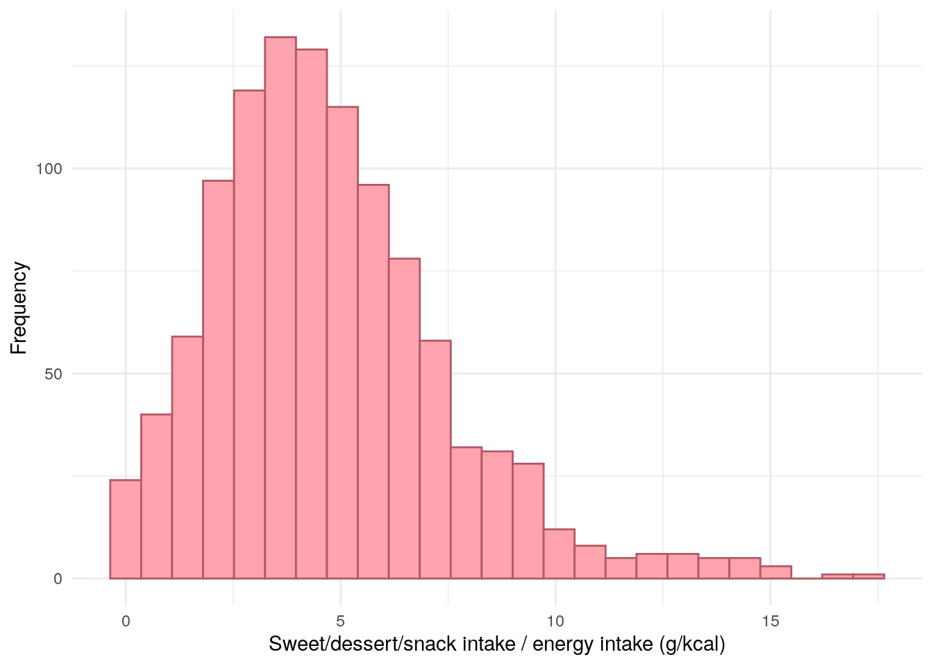
Figure 11: Distribution of Sweet and dessert/snack intake divided by daily energy intake.

Code

#| label: tbl-sweetintake-uc
#| tbl-cap: "ANOVA between sweet/dessert/snack intake intake and FC for UC/IBDU."

demo %>%
  filter(diagnosis2 == "UC/IBDU") %>%
  aov(formula = sweetIntake ~ cat) %>%
  summary() %>%
  pander()

Analysis of Variance Model
	Df	Sum Sq	Mean Sq	F value	Pr(>F)
cat	2	28.62	14.31	2.053	0.1294
Residuals	512	3569	6.971	NA	NA

Code

#| label: tbl-sweetIntake
#| tbl-cap: "ANOVA between sweet/dessert/snack intake and FC groups."
pander(summary(aov(sweetIntake ~ cat, data = demo)))

Analysis of Variance Model
	Df	Sum Sq	Mean Sq	F value	Pr(>F)
cat	2	1.351	0.6754	0.09064	0.9134
Residuals	1009	7518	7.451	NA	NA

Code

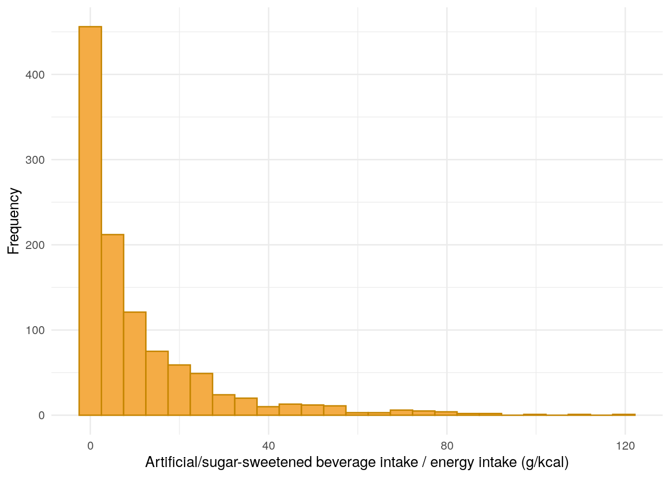
FFQ$drinkIntake <- with(FFQ,
                        (Beverages18h_grams + 
                          Beverages18i_grams +
                          Beverages18j_grams +
                          Beverages18k_grams +
                          Beverages18n_grams +
                          Beverages18o_grams) /
                          EnergykCAL) * 100

demo <- merge(demo,
              FFQ[, c("ParticipantNo", "drinkIntake")],
              by = "ParticipantNo",
              all.x = TRUE,
              all.y = FALSE)

demo %>%
  drop_na(drinkIntake) %>%
  ggplot(aes(x = drinkIntake)) +
  geom_histogram(bins = 25, color = "#C58500", fill = "#F4AC45") +
  theme_minimal() +
  xlab("Artificial/sugar-sweetened beverage intake / energy intake (g/kcal)") +
  ylab("Frequency")

Figure 12: Distribution of artificially and sugar-sweetened drink intake divided by daily energy intake.

Code

pander(summary(aov(sweetIntake ~ cat, data = demo)))

Table 14: ANOVA between artificial/sugar-sweetened beverage intake and FC groups.

Analysis of Variance Model
	Df	Sum Sq	Mean Sq	F value	Pr(>F)
cat	2	1.351	0.6754	0.09064	0.9134
Residuals	1009	7518	7.451	NA	NA

Code

FFQ$processedMeatIntake <- with(FFQ,
                                (meat7b_grams +
                                  meat7c_grams +
                                  meat7g_grams +
                                  meat7i_grams +
                                  meat7j_grams +
                                  meat7k_grams +
                                  meat7l_grams +
                                  fish8a_grams +
                                  fish8e_grams +
                                  fish8k_grams) /
                                  EnergykCAL) * 100

demo <- merge(demo,
              FFQ[, c("ParticipantNo", "processedMeatIntake")],
              by = "ParticipantNo",
              all.x = TRUE,
              all.y = FALSE)

demo %>%
  drop_na(processedMeatIntake) %>%
  ggplot(aes(x = processedMeatIntake)) +
  geom_histogram(bins = 25, color = "#BC0019", fill = "#FF4C55") +
  theme_minimal() +
  xlab("Processed animal-based product intake / energy intake (g/kcal)") +
  ylab("Frequency")

Figure 13: Distribution of processed animal-based product intake divided by daily energy intake.

Code

pander(summary(aov(processedMeatIntake ~ cat, data = demo)))

Table 15: ANOVA between processed meat intake and FC groups.

Analysis of Variance Model
	Df	Sum Sq	Mean Sq	F value	Pr(>F)
cat	2	27.23	13.62	6.328	0.001857
Residuals	1009	2171	2.152	NA	NA

From Figure 14, it appears subjects with FC<50μg/g at recruitment were more likely to consume no, or low levels of, processed meat.

Code

demo %>%
  drop_na(processedMeatIntake, cat) %>%
  ggplot(aes(x = processedMeatIntake)) +
  geom_histogram(bins = 25, color = "#BC0019", fill = "#FF4C55") +
  theme_minimal() +
  xlab("Processed animal-based product intake / energy intake (g/kcal)") +
  ylab("Frequency") +
  facet_grid(rows = vars(cat))

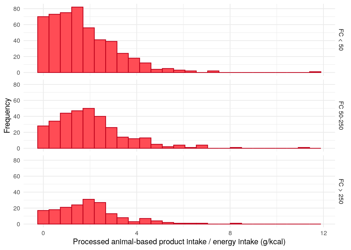
Figure 14: Distribution of processed animal-based product intake, divided by daily energy intake, and stratified by faecal calprotectin category.

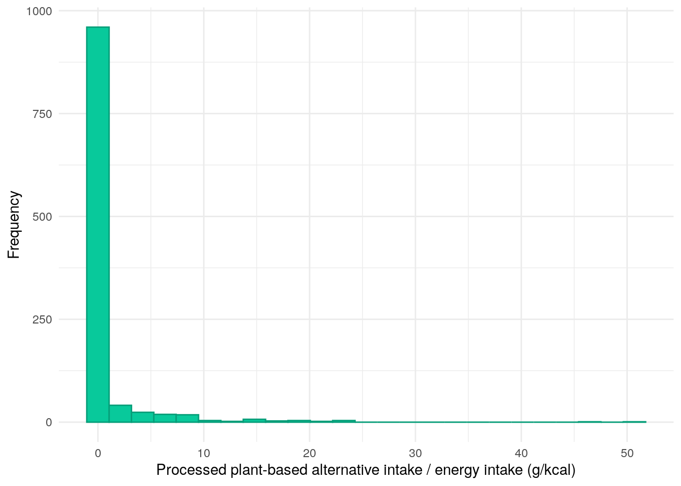
As one would likely expect, consumption of processed plant-based alternatives is low.

Code

FFQ$processedPlantIntake <- with(FFQ,
                                (Milk3d_grams +
                                   Sav_etc10d_grams +
                                   Sav_etc10e_grams +
                                   Sav_etc10f_grams) /
                                  EnergykCAL) * 100

demo <- merge(demo,
              FFQ[, c("ParticipantNo", "processedPlantIntake")],
              by = "ParticipantNo",
              all.x = TRUE,
              all.y = FALSE)

demo %>%
  drop_na(processedPlantIntake) %>%
  ggplot(aes(x = processedPlantIntake)) +
  geom_histogram(bins = 25, color = "#069E79", fill = "#08C99B") +
  theme_minimal() +
  xlab("Processed plant-based alternative intake / energy intake (g/kcal)") +
  ylab("Frequency")

Figure 15: Distribution of processed plant-based alternatives divided by daily energy intake.

Code

pander(summary(aov(processedPlantIntake ~ cat, data = demo)))

Table 16: ANOVA between processed plant-based alternatives intake and FC groups.

Analysis of Variance Model
	Df	Sum Sq	Mean Sq	F value	Pr(>F)
cat	2	11.35	5.675	0.4328	0.6488
Residuals	1009	13230	13.11	NA	NA

Un-processed/minimally processed food subgroups

Code

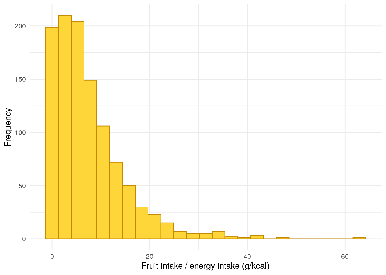
FFQ$fruitIntake <- with(FFQ,
                        (fruit12a_grams + 
                           fruit12b_grams +
                           fruit12c_grams +
                           fruit12c_grams +
                           fruit12f_grams +
                           fruit12g_grams +
                           fruit12h_grams +
                           fruit12i_grams +
                           fruit12j_grams) /
                         EnergykCAL) * 100
demo <- merge(demo,
              FFQ[, c("ParticipantNo", "fruitIntake")],
              by = "ParticipantNo",
              all.x = TRUE,
              all.y = FALSE)

demo %>%
  drop_na(fruitIntake) %>%
  ggplot(aes(x = fruitIntake)) +
  geom_histogram(bins = 25, color =  "#C58901", fill = "#FFD639") +
  theme_minimal() +
  xlab("Fruit intake / energy intake (g/kcal)") +
  ylab("Frequency")

Figure 16: Distribution of fruit intake divided by daily energy intake.

Code

pander(summary(aov(fruitIntake ~ cat, data = demo)))

Table 17: ANOVA between fruit intake and FC groups.

Analysis of Variance Model
	Df	Sum Sq	Mean Sq	F value	Pr(>F)
cat	2	193.2	96.59	1.821	0.1624
Residuals	1009	53513	53.04	NA	NA

Code

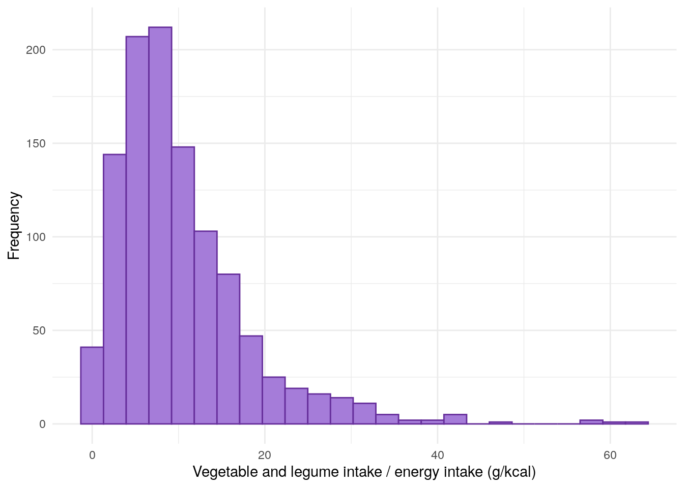
FFQ$vegIntake <- with(FFQ,
                        (Veg11a_grams + 
                           Veg11b_grams + 
                           Veg11c_grams + 
                           Veg11d_grams +
                           Veg11e_grams +
                           Veg11f_grams + 
                           Veg11g_grams +
                           Veg11h_grams +
                           Veg11i_grams + 
                           Veg11j_grams +
                           Veg11k_grams + 
                           Veg11l_grams + 
                           Veg11m_grams + 
                           Veg11n_grams + 
                           Veg11o_grams + 
                           Veg11p_grams +
                           Pulses) /
                         EnergykCAL) * 100
demo <- merge(demo,
              FFQ[, c("ParticipantNo", "vegIntake")],
              by = "ParticipantNo",
              all.x = TRUE,
              all.y = FALSE)

demo %>%
  drop_na(vegIntake) %>%
  ggplot(aes(x = vegIntake)) +
  geom_histogram(bins = 25, color =  "#662E9B", fill = "#A57CD9") +
  theme_minimal() +
  xlab("Vegetable and legume intake / energy intake (g/kcal)") +
  ylab("Frequency")

Figure 17: Distribution of vegetable and legume intake divided by daily energy intake.

Code

pander(summary(aov(vegIntake ~ cat, data = demo)))

Table 18: ANOVA between vegetable/legume intake and FC groups.

Analysis of Variance Model
	Df	Sum Sq	Mean Sq	F value	Pr(>F)
cat	2	335.3	167.6	2.71	0.06702
Residuals	1006	62228	61.86	NA	NA

Code

FFQ$redMeatIntake <- with(FFQ,
                        (meat7d_grams + 
                           meat7e_grams + 
                           meat7h_grams) /
                         EnergykCAL) * 100
demo <- merge(demo,
              FFQ[, c("ParticipantNo", "redMeatIntake")],
              by = "ParticipantNo",
              all.x = TRUE,
              all.y = FALSE)

demo %>%
  drop_na(redMeatIntake) %>%
  ggplot(aes(x = redMeatIntake)) +
  geom_histogram(bins = 25, color =  "#93250B", fill = "#F34213") +
  theme_minimal() +
  xlab("VRed meat intake / energy intake (g/kcal)") +
  ylab("Frequency")

Figure 18: Distribution of red meat intake divided by daily energy intake.

Code

pander(summary(aov(redMeatIntake ~ cat, data = demo)))

Table 19: ANOVA between red meat intake and FC groups.

Analysis of Variance Model
	Df	Sum Sq	Mean Sq	F value	Pr(>F)
cat	2	0.2782	0.1391	0.1716	0.8424
Residuals	1009	818	0.8107	NA	NA

Code

FFQ$whiteMeatIntake <- with(FFQ,
                            meat7f_grams /
                              EnergykCAL) * 100
demo <- merge(demo,
              FFQ[, c("ParticipantNo", "whiteMeatIntake")],
              by = "ParticipantNo",
              all.x = TRUE,
              all.y = FALSE)

demo %>%
  drop_na(whiteMeatIntake) %>%
  ggplot(aes(x = whiteMeatIntake)) +
  geom_histogram(bins = 25, color =  "#829399", fill = "#545F66") +
  theme_minimal() +
  xlab("White meat intake / energy intake (g/kcal)") +
  ylab("Frequency")

Figure 19: Distribution of white/oily fish intake divided by daily energy intake.

Code

pander(summary(aov(whiteMeatIntake ~ cat, data = demo)))

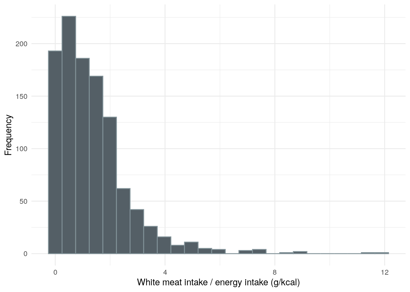
Table 20: ANOVA between white meat intake and FC groups.

Analysis of Variance Model
	Df	Sum Sq	Mean Sq	F value	Pr(>F)
cat	2	3.262	1.631	0.8655	0.4212
Residuals	1009	1901	1.884	NA	NA

Code

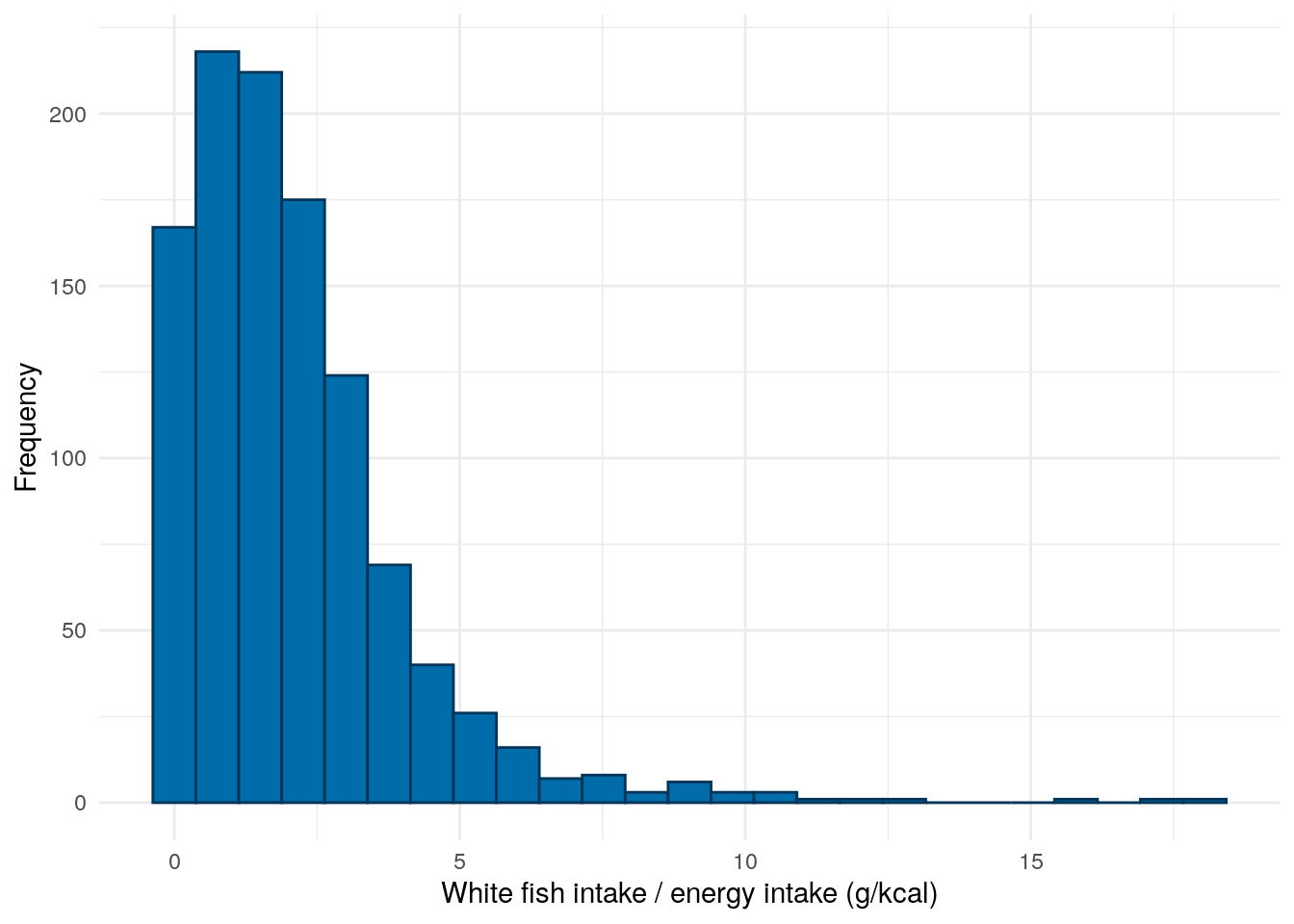
FFQ$whiteFishIntake <- with(FFQ,
                        (WhiteFish + 
                           OilyFish) /
                         EnergykCAL) * 100
demo <- merge(demo,
              FFQ[, c("ParticipantNo", "whiteFishIntake")],
              by = "ParticipantNo",
              all.x = TRUE,
              all.y = FALSE)

demo %>%
  drop_na(whiteFishIntake) %>%
  ggplot(aes(x = whiteFishIntake)) +
  geom_histogram(bins = 25, color =  "#003559", fill = "#006DAA") +
  theme_minimal() +
  xlab("White fish intake / energy intake (g/kcal)") +
  ylab("Frequency")

Figure 20: Distribution of white/oily fish intake divided by daily energy intake.

Code

pander(summary(aov(whiteFishIntake ~ cat, data = demo)))

Table 21: ANOVA between fish (white and oily) intake and FC groups.

Analysis of Variance Model
	Df	Sum Sq	Mean Sq	F value	Pr(>F)
cat	2	8.924	4.462	1.089	0.3369
Residuals	1003	4109	4.097	NA	NA

Percentage of energy intake

Code

nova4 <- read_xlsx(paste0(upf.path, "NOVA4Scores.xlsx"))
colnames(nova4)[c(1, 6)] <- c("ParticipantNo", "UPF_perc")
demo <- merge(demo,
  nova4[, c("ParticipantNo", "UPF_perc")],
  by = "ParticipantNo",
  all.x = TRUE,
  all.y = FALSE
)

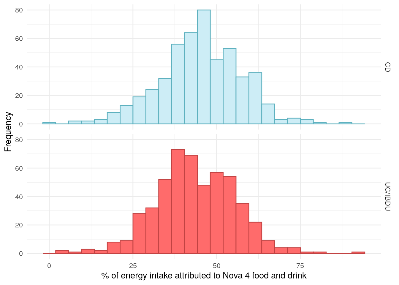
As an alternative to the above analyses, we have also explored the percentage of daily energy intake which is derived from ultra processed (UPF4) groups.

Code

demo %>%
  drop_na(cat) %>%
  ggplot(aes(x = UPF_perc, color = diagnosis2, fill = diagnosis2)) +
  geom_histogram(bins = 25) +
  theme_minimal() +
  theme(legend.position = "none") +
  labs(
    x = "% of energy intake attributed to Nova 4 food and drink",
    y = "Frequency",
    color = "IBD type",
    fill = "IBD type"
  ) +
  scale_fill_manual(
    values = c("#CDEDF6", "#FF6B6B")
  ) +
  scale_color_manual(
    values = c("#5EB1BF", "#C24343")
  ) +
  facet_grid(rows = vars(diagnosis2))

Warning: Removed 1132 rows containing non-finite outside the scale range
(`stat_bin()`).

Figure 21: Distribution of the percentage of daily energy intake sourced from UPF (Nova score 4) food and drink.

Code

demo %>%
  filter(diagnosis2 == "CD") %>%
  aov(formula = UPF_perc ~ cat) %>%
  summary() %>%
  pander()

Table 22: ANOVA between Nova 4 food as a percentage of energy intake and FC for Crohn’s diseease.

Analysis of Variance Model
	Df	Sum Sq	Mean Sq	F value	Pr(>F)
cat	2	242.9	121.4	0.7854	0.4565
Residuals	494	76379	154.6	NA	NA

Code

demo %>%
  filter(diagnosis2 == "UC/IBDU") %>%
  aov(formula = UPF_perc ~ cat) %>%
  summary() %>%
  pander()

Table 23: ANOVA between Nova 4 food as a percentage of energy intake and FC for UC/IBDU.

Analysis of Variance Model
	Df	Sum Sq	Mean Sq	F value	Pr(>F)
cat	2	1357	678.4	4.822	0.008423
Residuals	512	72042	140.7	NA	NA

Code

p <- demo %>%
  filter(diagnosis2 == "UC/IBDU") %>%
  drop_na(cat, UPF_perc) %>%
  mutate(cat = fct_rev(cat)) %>%
  ggplot(aes(x = UPF_perc, fill = cat, color = cat)) +
  geom_density() +
  facet_grid(rows = vars(cat)) +
  labs(x = "Nova 4 food as a percentage of energy intake",
       y = "Density",
       fill = "FC group",
       color = "FC group")
cat_theme(p)

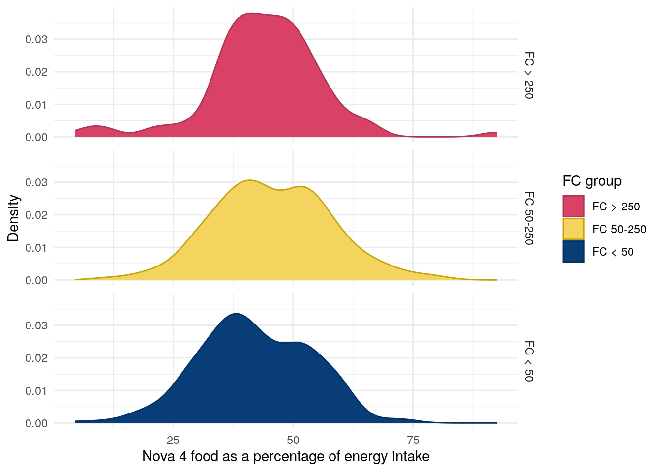
Figure 22: Distribution of Nova 4 food as a percentage of energy intake by FC in UC.

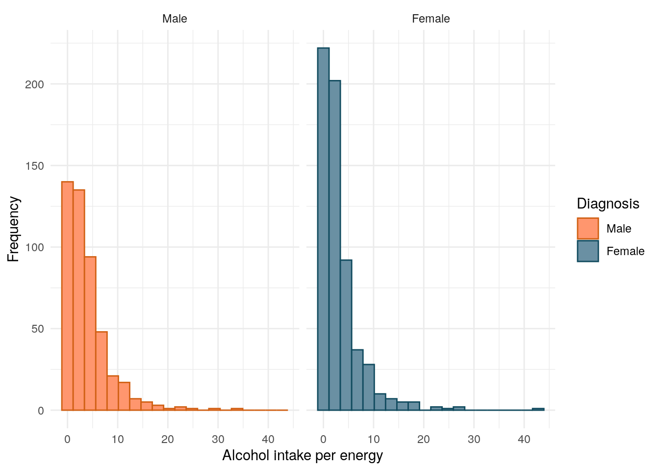
Alcohol use

Code

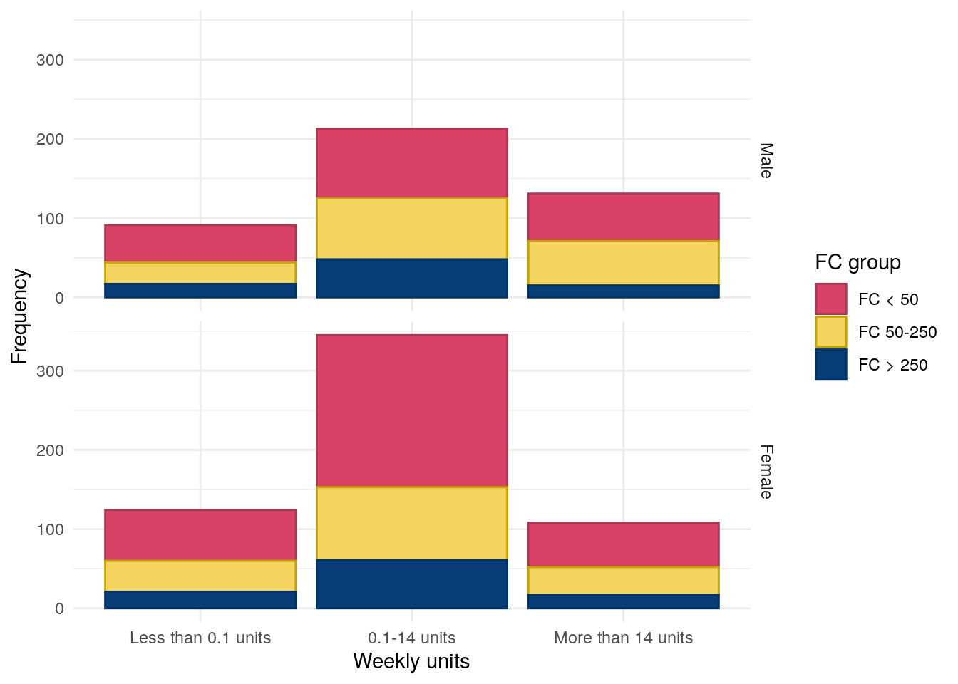
demo <- FFQ %>%
  select(ParticipantNo,
         Alcoholg,
         Alcohol_percEng,
         Alcohol_units,
         Alcohol_units_wk) %>%
  merge(x = demo,
        by = "ParticipantNo",
        all.x = TRUE,
        all.y = FALSE)

demo %<>% mutate(
    weekly_units_cat = case_when(
      Alcohol_units_wk <= 0.1 ~ "Less than 0.1 units",
      Alcohol_units_wk > 0.1 & Alcohol_units_wk <= 14 ~ "0.1-14 units",
      Alcohol_units_wk > 14 ~ "More than 14 units"
    )
  ) %>%
  mutate(weekly_units_cat = factor(
    weekly_units_cat,
    levels = c("Less than 0.1 units", "0.1-14 units", "More than 14 units")
))

For alcohol usage we consider both alcohol intake as a percentage of energy intake and weekly alcohol units, categorised into 0-0.1, 0.1-14 and more than 14 units per week.

Weekly alcohol units

Code

p <- demo %>%
  drop_na(weekly_units_cat, cat) %>%
  ggplot(aes(x = weekly_units_cat, color = cat, fill = cat)) +
  geom_bar() +
  facet_grid(rows = vars(Sex)) +
  labs(x = "Weekly units",
       y = "Frequency", 
       color = "FC group",
       fill = "FC group") +
  theme_minimal()
cat_theme(p)

Figure 23: Distribution of weekly alcohol units, stratified by sex.

Code

pander(chisq.test(temp$NOVAScore_cat, temp$cat))

Table 24: Chi-squared test between weekly alcohol units and FC groups.

Pearson’s Chi-squared test: `temp$NOVAScore_cat` and `temp$cat`
Test statistic	df	P value
4.197	6	0.6501

Percentage of energy

Code

demo %>%
  drop_na(Alcohol_percEng) %>%
  ggplot(aes(x = Alcohol_percEng, color = Sex, fill = Sex)) +
  geom_histogram(bins = 20) +
  facet_grid(cols = vars(Sex)) + 
  theme_minimal() +
  labs(x = "Alcohol intake per energy",
       y = "Frequency",
       color = "Diagnosis",
       fill = "Diagnosis") +
  scale_fill_manual(values = c("#FF966E", "#6A90A3")) +
  scale_color_manual(values = c("#D16014",  "#114B5F"))

Figure 24: Distribution of alcohol intake per energy, stratified by sex.

Code

pander(summary(aov(Alcohol_percEng ~ cat, data = demo)))

Table 25: ANOVA between alcohol intake and FC groups.

Analysis of Variance Model
	Df	Sum Sq	Mean Sq	F value	Pr(>F)
cat	2	60.53	30.26	1.624	0.1977
Residuals	1009	18806	18.64	NA	NA

Diet quality index

Code

demo %>%
  drop_na(dqi_tot) %>%
  ggplot(aes(x = dqi_tot, color = diagnosis2, fill = diagnosis2)) +
  geom_histogram(bins = 20) +
  facet_grid(cols = vars(diagnosis2)) + 
  theme_minimal() +
  labs(x = "Diet quality index",
       y = "Frequency",
       color = "Diagnosis",
       fill = "Diagnosis") +
  scale_fill_manual(values = c("#86DEB7", "#FC5A66")) +
  scale_color_manual(values = c("#529176",  "#AC353F"))

Figure 25: Distribution of diet quality index, stratified by IBD type.

Code

demo %>%
  drop_na(dqi_tot, cat) %>%
  pull(dqi_tot) %>%
  quantile() %>%
  knitr::kable(digits = 2,
    caption = "Diet quality index quantiles for the FFQ subcohort.",
    col.names = c("Quantile", "DQI")
  )

Diet quality index quantiles for the FFQ subcohort.
Quantile	DQI
0%	5.59
25%	26.60
50%	33.99
75%	41.36
100%	60.00

Code

pander(summary(aov(dqi_tot ~ cat, data = demo)))

Table 26: ANOVA between diet quality index and FC groups.

Analysis of Variance Model
	Df	Sum Sq	Mean Sq	F value	Pr(>F)
cat	2	676.6	338.3	2.818	0.06019
Residuals	1009	121118	120	NA	NA

Code

saveRDS(demo, paste0(outdir, "demo-diet.RDS"))

Comparison

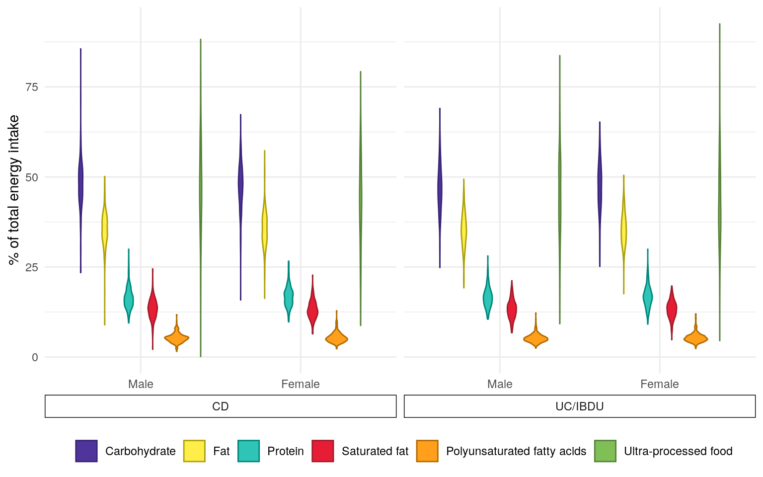
Figure 26 presents macronutrient, PUFA and UPF intake as percentages of total energy intake.

Code

FFQ$Prot_percEng <- ((FFQ$Protng * 4) / FFQ$EnergykCAL) * 100

FFQ <- merge(FFQ,
  nova4[, c("ParticipantNo", "UPF_perc")],
  by = "ParticipantNo",
  all.x = TRUE,
  all.y = FALSE
)


comparison <- reshape2::melt(FFQ,
  id.vars = "ParticipantNo",
  measure.vars = c(
    "CHO_percEng",
    "Fat_percEng",
    "Prot_percEng",
    "SatFat_percEng",
    "PUFA_percEng",
    "UPF_perc"
  )
)

comparison <- merge(comparison,
  demo[, c("ParticipantNo", "Sex", "diagnosis2")],
  by = "ParticipantNo",
  all.x = TRUE,
  all.y = FALSE
)

comparison$variable <- factor(comparison$variable,
  levels = c(
    "CHO_percEng",
    "Fat_percEng",
    "Prot_percEng",
    "SatFat_percEng",
    "PUFA_percEng",
    "UPF_perc"
  ),
  labels = c(
    "Carbohydrate",
    "Fat",
    "Protein",
    "Saturated fat",
    "Polyunsaturated fatty acids",
    "Ultra-processed food"
  ))

p <- ggplot(
  comparison,
  aes(color = variable, fill = variable, y = value, x = Sex)
) +
  geom_violin() +
  facet_grid(~diagnosis2,
    scales = "free_x",
    space = "free_x",
    switch = "x"
  ) +
  theme_minimal() +
  theme(
    strip.placement = "outside",
    strip.background = element_rect(fill = "white"),
    strip.clip = "on",
    axis.title.x = element_blank(),
    legend.position = "bottom"
  ) +
  scale_fill_manual(
    values = c(
      "#4F359B",
      "#FFED49",
      "#2EC4B6",
      "#E71D36",
      "#FF9F1C",
      "#80BF56"
    )
  ) +
  scale_color_manual(
    values = c(
      "#392376",
      "#ADA009",
      "#00877C",
      "#9F1C29",
      "#B06B01",
      "#568238"
    )
  ) +
  labs(
    y = "% of total energy intake",
    color = "",
    fill = ""
  ) + guides(
    colour = guide_legend(nrow = 1),
    fill = guide_legend(nrow = 1))

ggsave("plots/baseline/diet.png", p, width = 12 * 0.8, height = 7 * 0.8)
ggsave("plots/baseline/diet.pdf", p, width = 12 * 0.8, height = 7 * 0.8)
p

Figure 26: Dietary distribution of the FFQ subcohort expressed as percentages of energy intake and stratified by sex and diagnosis of either Crohn’s disease or ulcerative colitis/inflammatory bowel disease unclassified.

Missingness

Code

demo %>%
  filter(ParticipantNo %in% FFQ$ParticipantNo) %>%
  select(
  Meat_sum,
  meat_overall,
  fish_overall,
  fibre,
  PUFA_percEng,
  NOVAScore_cat,
  dqi_tot,
  breadIntake,
  sweetIntake,
  drinkIntake,
  processedMeatIntake,
  processedPlantIntake,
  fruitIntake,
  vegIntake,
  redMeatIntake,
  whiteMeatIntake,
  whiteFishIntake,
  UPF_perc,
  Alcohol_percEng, 
  SiteName
  ) %>%
missing_plot2(title = "Disease phenotyping missingness")

Reproduction and reproducibility

Session info

R version 4.4.0 (2024-04-24)

Platform: aarch64-unknown-linux-gnu

locale: LC_CTYPE=en_US.UTF-8, LC_NUMERIC=C, LC_TIME=en_US.UTF-8, LC_COLLATE=en_US.UTF-8, LC_MONETARY=en_US.UTF-8, LC_MESSAGES=en_US.UTF-8, LC_PAPER=en_US.UTF-8, LC_NAME=C, LC_ADDRESS=C, LC_TELEPHONE=C, LC_MEASUREMENT=en_US.UTF-8 and LC_IDENTIFICATION=C

attached base packages: stats, graphics, grDevices, utils, datasets, methods and base

other attached packages: DiagrammeRsvg(v.0.1), DiagrammeR(v.1.0.11), pander(v.0.6.5), knitr(v.1.47), table1(v.1.4.3), patchwork(v.1.2.0), datefixR(v.1.6.1), readxl(v.1.4.3), lubridate(v.1.9.3), forcats(v.1.0.0), stringr(v.1.5.1), dplyr(v.1.1.4), purrr(v.1.0.2), readr(v.2.1.5), tidyr(v.1.3.1), tibble(v.3.2.1), ggplot2(v.3.5.1), tidyverse(v.2.0.0) and plyr(v.1.8.9)

loaded via a namespace (and not attached): shape(v.1.4.6.1), gtable(v.0.3.5), xfun(v.0.44), htmlwidgets(v.1.6.4), visNetwork(v.2.1.2), lattice(v.0.22-6), tzdb(v.0.4.0), vctrs(v.0.6.5), tools(v.4.4.0), generics(v.0.1.3), curl(v.5.2.1), fansi(v.1.0.6), pan(v.1.9), jomo(v.2.7-6), pkgconfig(v.2.0.3), Matrix(v.1.7-0), RColorBrewer(v.1.1-3), lifecycle(v.1.0.4), compiler(v.4.4.0), farver(v.2.1.2), textshaping(v.0.4.0), munsell(v.0.5.1), codetools(v.0.2-20), htmltools(v.0.5.8.1), yaml(v.2.3.8), finalfit(v.1.0.7), glmnet(v.4.1-8), Formula(v.1.2-5), mice(v.3.16.0), nloptr(v.2.0.3), pillar(v.1.9.0), MASS(v.7.3-60.2), iterators(v.1.0.14), rpart(v.4.1.23), boot(v.1.3-30), mitml(v.0.4-5), foreach(v.1.5.2), nlme(v.3.1-164), tidyselect(v.1.2.1), digest(v.0.6.35), stringi(v.1.8.4), reshape2(v.1.4.4), splines(v.4.4.0), labeling(v.0.4.3), fastmap(v.1.2.0), grid(v.4.4.0), colorspace(v.2.1-0), cli(v.3.6.2), magrittr(v.2.0.3), survival(v.3.5-8), utf8(v.1.2.4), broom(v.1.0.6), withr(v.3.0.0), scales(v.1.3.0), backports(v.1.5.0), timechange(v.0.3.0), rmarkdown(v.2.27), nnet(v.7.3-19), lme4(v.1.1-35.3), cellranger(v.1.1.0), ragg(v.1.3.2), hms(v.1.1.3), evaluate(v.0.23), V8(v.4.4.2), rlang(v.1.1.3), Rcpp(v.1.0.12), glue(v.1.7.0), minqa(v.1.2.7), jsonlite(v.1.8.8), R6(v.2.5.1) and systemfonts(v.1.3.1)

Licensed by CC BY unless otherwise stated.

References

Ananthakrishnan, Ashwin N., Hamed Khalili, Gauree G. Konijeti, Leslie M. Higuchi, Punyanganie de Silva, Joshua R. Korzenik, Charles S. Fuchs, Walter C. Willett, James M. Richter, and Andrew T. Chan. 2013. “A Prospective Study of Long-Term Intake of Dietary Fiber and Risk of Crohn’s Disease and Ulcerative Colitis.” Gastroenterology 145 (5): 970–77. https://doi.org/10.1053/j.gastro.2013.07.050.

Brotherton, Carol S., Christopher A. Martin, Millie D. Long, Michael D. Kappelman, and Robert S. Sandler. 2016. “Avoidance of Fiber Is Associated with Greater Risk of Crohn’s Disease Flare in a 6-Month Period.” Clinical Gastroenterology and Hepatology 14 (8): 1130–36. https://doi.org/10.1016/j.cgh.2015.12.029.

Cordova, Reynalda, Vivian Viallon, Emma Fontvieille, Laia Peruchet-Noray, Anna Jansana, Karl-Heinz Wagner, Cecilie Kyrø, et al. 2023. “Consumption of Ultra-Processed Foods and Risk of Multimorbidity of Cancer and Cardiometabolic Diseases: A Multinational Cohort Study.” The Lancet Regional Health - Europe 35 (December): 100771. https://doi.org/10.1016/j.lanepe.2023.100771.

Kim, Soowon, Pamela S. Haines, Anna Maria Siega-Riz, and Barry M. Popkin. 2003. “The Diet Quality Index-International (DQI-i) Provides an Effective Tool for Cross-National Comparison of Diet Quality as Illustrated by China and the United States.” The Journal of Nutrition 133 (11): 3476–84. https://doi.org/10.1093/jn/133.11.3476.

Marion-Letellier, Rachel, Guillaume Savoye, Beck Paul L., Remo Panaccione, and Subrata Ghosh. 2013. “Polyunsaturated Fatty Acids in Inflammatory Bowel Diseases: A Reappraisal of Effects and Therapeutic Approaches.” Inflammatory Bowel Diseases 19 (3): 650–61. https://doi.org/10.1097/mib.0b013e3182810122.

Monteiro, Carlos Augusto, Geoffrey Cannon, Jean-Claude Moubarac, Renata Bertazzi Levy, Maria Laura C Louzada, and Patrícia Constante Jaime. 2017. “The UN Decade of Nutrition, the NOVA Food Classification and the Trouble with Ultra-Processing.” Public Health Nutrition 21 (1): 5–17. https://doi.org/10.1017/s1368980017000234.

Narula, Neeraj, Emily C L Wong, Mahshid Dehghan, Andrew Mente, Sumathy Rangarajan, Fernando Lanas, Patricio Lopez-Jaramillo, et al. 2021. “Association of Ultra-Processed Food Intake with Risk of Inflammatory Bowel Disease: Prospective Cohort Study.” BMJ, July, n1554. https://doi.org/10.1136/bmj.n1554.