set.seed(123)suppressPackageStartupMessages(library(tidyverse))# ggplot2, dplyr, and magrittrlibrary(readxl)# Read in Excel files# Generate flowchart of cohort derivationlibrary(DiagrammeR)library(DiagrammeRsvg)if(file.exists("/docker")){# If running in dockerdata.path<-"data/final/20221004/"redcap.path<-"data/final/20231030/"prefix<-"data/end-of-follow-up/"outdir<-"data/processed/"metadir<-"data/metadata/"}else{# Run on OS directlydata.path<-"/Volumes/igmm/cvallejo-predicct/predicct/final/20221004/"redcap.path<-"/Volumes/igmm/cvallejo-predicct/predicct/final/20231030/"prefix<-"/Volumes/igmm/cvallejo-predicct/predicct/end-of-follow-up/"outdir<-"/Volumes/igmm/cvallejo-predicct/predicct/processed/"metadir<-"/Volumes/igmm/cvallejo-predicct/predicct/metadata/"}eof<-read_xlsx(paste0(prefix, "Followup form.xlsx"))# Demographic data as reported by subjectsdemo<-read_xlsx(paste0(data.path, "Baseline2022/demographics.xlsx"), col_types =c("text","text","text","text","numeric","numeric","text","text","date","numeric","text"))
Country of recruitment
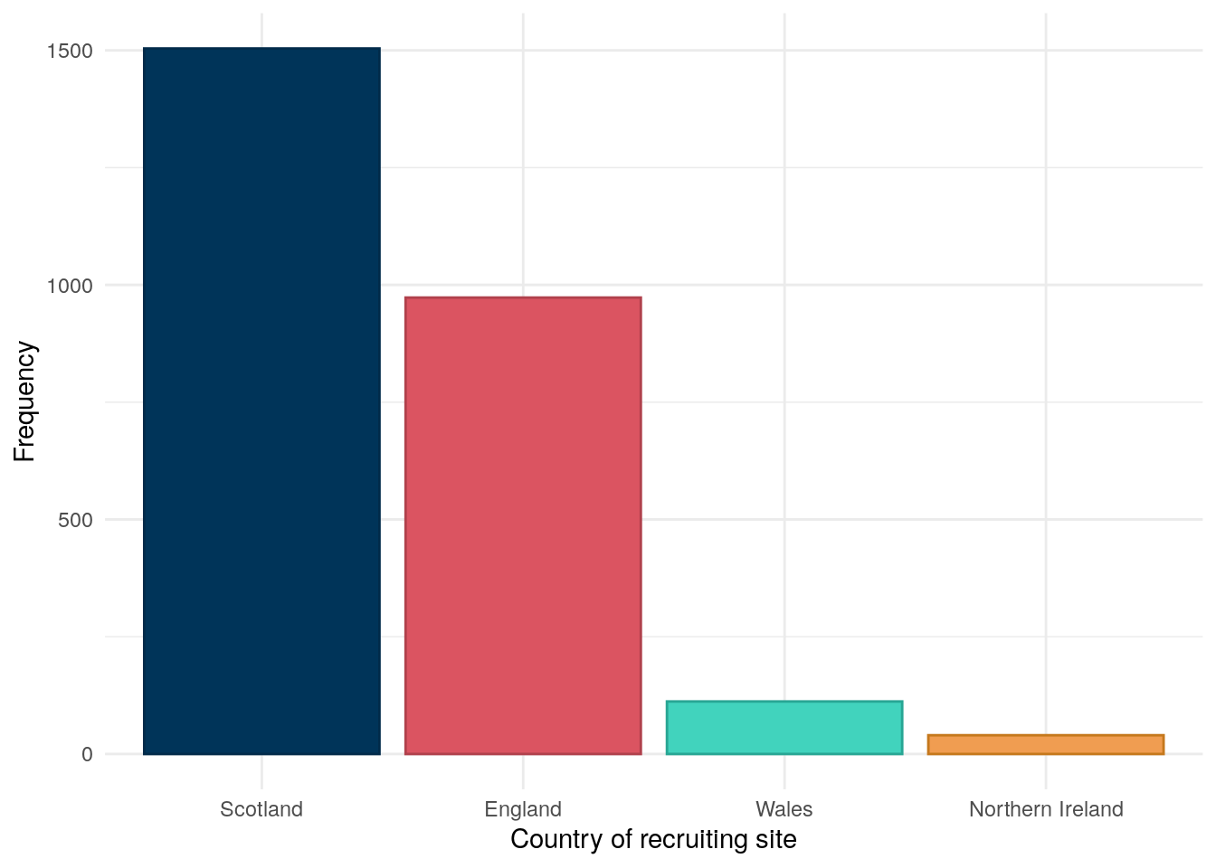
PREdiCCt is a pan-UK study which recruited across 47 sites. Figure 1 shows the distribution of the PREdiCCt cohort by country of the recruiting site.
Code
site.data<-read.csv(paste0(metadir, "sites.csv"))sites<-demo%>%select(ParticipantNo, SiteNo)sites<-merge(sites, site.data, by ="SiteNo", all.x =TRUE, all.y =FALSE)plt.cols<-c("#003459", "#DB5461", "#41D3BD", "#F09D51")sites$Country<-factor(sites$Country, levels =c("Scotland","England","Wales","Northern Ireland"))sites%>%ggplot(aes(x =Country, color =Country, fill =Country))+geom_bar()+theme_minimal()+theme(legend.position ="none")+xlab("Country of recruiting site")+ylab("Frequency")+scale_fill_manual(values =plt.cols)+scale_color_manual(values =colorspace::darken(plt.cols, 0.2))
Figure 1: Distribution of the PREdiCCt cohort by country of recruitment site.
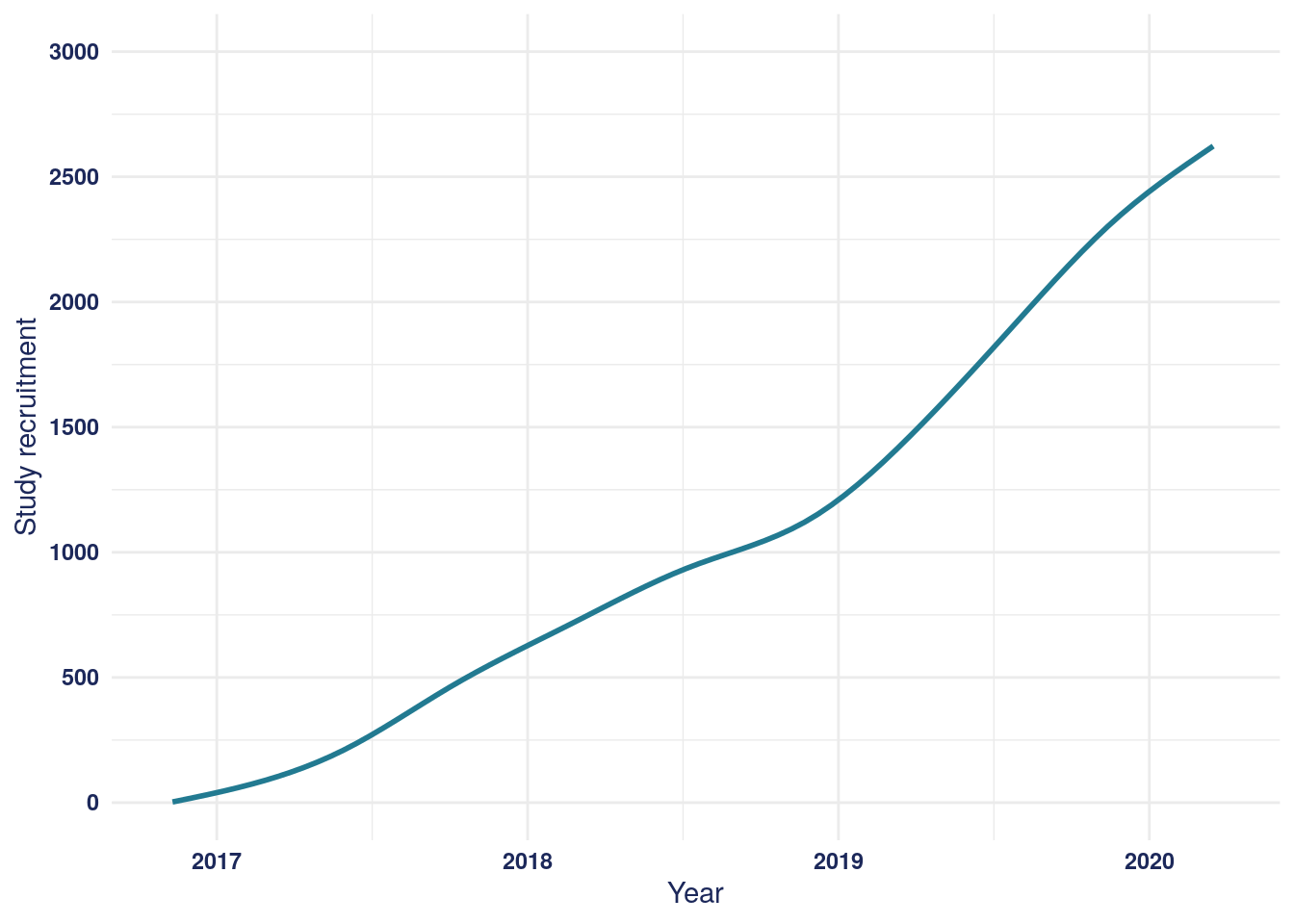
Recruitment to PREdiCCt began in November 2016. As participants were recruited when they attended IBD clinic appointments and the COVID-19 pandemic substantially decreased the number of in-person clinic appointments, recruitment was ceased in March 2020.
Figure 2: Cumulative recruitment to the PREdiCCt study over time.
Month of recruitment
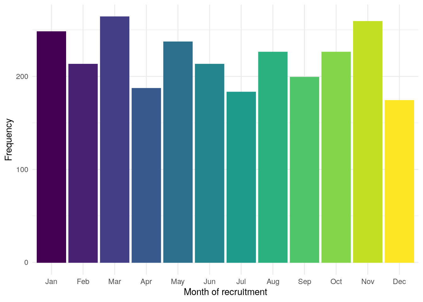
There is potential for seasonality to confound interpretations of our results, particularly when making inferences regarding diet. As such, month of recruitment is explored (Figure 3).
Recruitment was low in December, which is to be as expected as there are typically fewer clinic appointments in December and participants were recruited in IBD clinics.
However, recruitment was also low in April and July. As such, the impact of seasonality is likely to be minimal for this cohort and will be ignored for all analyses.
---title: "Study recruitment"author: - name: "Nathan Constantine-Cooke" corresponding: true url: https://scholar.google.com/citations?user=2emHWR0AAAAJ&hl=en&oi=ao affiliations: - ref: IGCbibliography: Baseline.bib ---```{R}set.seed(123)suppressPackageStartupMessages(library(tidyverse)) # ggplot2, dplyr, and magrittrlibrary(readxl) # Read in Excel files# Generate flowchart of cohort derivationlibrary(DiagrammeR)library(DiagrammeRsvg)if (file.exists("/docker")) { # If running in docker data.path <-"data/final/20221004/" redcap.path <-"data/final/20231030/" prefix <-"data/end-of-follow-up/" outdir <-"data/processed/" metadir <-"data/metadata/"} else { # Run on OS directly data.path <-"/Volumes/igmm/cvallejo-predicct/predicct/final/20221004/" redcap.path <-"/Volumes/igmm/cvallejo-predicct/predicct/final/20231030/" prefix <-"/Volumes/igmm/cvallejo-predicct/predicct/end-of-follow-up/" outdir <-"/Volumes/igmm/cvallejo-predicct/predicct/processed/" metadir <-"/Volumes/igmm/cvallejo-predicct/predicct/metadata/"}eof <-read_xlsx(paste0(prefix, "Followup form.xlsx"))# Demographic data as reported by subjectsdemo <-read_xlsx(paste0(data.path, "Baseline2022/demographics.xlsx"),col_types =c("text","text","text","text","numeric","numeric","text","text","date","numeric","text" ))```### Country of recruitmentPREdiCCt is a pan-UK study which recruited across`r length(unique(demo$SiteName))` sites. @fig-country shows the distribution ofthe PREdiCCt cohort by country of the recruiting site. ```{R}#| label: fig-country#| fig-cap: "Distribution of the PREdiCCt cohort by country of recruitment site."site.data <-read.csv(paste0(metadir, "sites.csv"))sites <- demo %>%select(ParticipantNo, SiteNo)sites <-merge(sites, site.data, by ="SiteNo", all.x =TRUE, all.y =FALSE)plt.cols <-c( "#003459", "#DB5461", "#41D3BD", "#F09D51")sites$Country <-factor(sites$Country,levels =c("Scotland","England","Wales","Northern Ireland"))sites %>%ggplot(aes(x = Country, color = Country, fill = Country)) +geom_bar() +theme_minimal() +theme(legend.position ="none") +xlab("Country of recruiting site") +ylab("Frequency") +scale_fill_manual(values = plt.cols) +scale_color_manual(values = colorspace::darken(plt.cols, 0.2))```### Recruitment over time```{R}demo <- demo %>%mutate(entry_date =as.Date(entry_date))```Recruitment to PREdiCCt began in November 2016. As participants wererecruited when they attended IBD clinic appointments and the COVID-19pandemic substantially decreased the number of in-person clinic appointments, recruitment was ceased in March 2020. ```{R}#| label: fig-recruitment#| fig-cap: "Cumulative recruitment to the PREdiCCt study over time."#| message: falsedemo_cumulative <- demo %>%arrange(entry_date) %>%mutate(cumulative_count =row_number())p <- demo_cumulative %>%ggplot(aes(x = entry_date, y = cumulative_count)) +geom_smooth(color =rgb(34, 122, 145, maxColorValue =255),method ="gam") +theme_minimal() +xlab("Year") +ylab("Study recruitment") +xlim(as.Date("2016-11-01"), as.Date("2020-04-01")) +scale_y_continuous(breaks =seq(0, 3000, by =500), limits =c(0, 3000)) +theme(text =element_text(color ="#1C285A"),axis.text =element_text(face ="bold", color ="#1C285A"))#ggsave("src/plots/baseline/cumulative-recruitment.png",# p,# width = 9 * 0.8,# height = 6 * 0.8)#ggsave("src/plots/baseline/cumulative-recruitment.pdf",# p,# width = 9 * 0.8,# height = 6 * 0.8)p```### Month of recruitmentThere is potential for seasonality to confound interpretations of our results,particularly when making inferences regarding diet. As such,month of recruitment is explored ([@fig-month]).Recruitment was low in December, which is to be as expected as there aretypically fewer clinic appointments in December and participants were recruitedin IBD clinics.However, recruitment was also low in April and July. As such, the impact ofseasonality is likely to be minimal for this cohort and will be ignored for allanalyses. ```{R}#| label: fig-month#| fig-cap: "Distribution of month of diagnosis."demo$entry_date <-as.Date(demo$entry_date)demo$month <-month(demo$entry_date, label =TRUE)ggplot(demo, aes(x =as.factor(month), color =as.factor(month), fill =as.factor(month))) +geom_bar() +theme_minimal() +theme(legend.position ="none") +xlab("Month of recruitment") +ylab("Frequency")```### Cohort derivationThe below flowchart gives a simple explanation of how the sub-cohort of subjectswith analysed food frequency questionnaires (FFQs) was obtained. ```{R}#| class-output: outputfcal <-read_xlsx(paste0(data.path, "Baseline2022/calprotectin.xlsx"))fcal$Result <-as.numeric(plyr::mapvalues(fcal$Result, from ="<20", to =20))fcal <- fcal[, c("ParticipantNo", "Result")]fcal.eof <-read_xlsx(paste0(prefix, "EOF_fcal.xlsx"))fcal.eof <-subset(fcal.eof, IsBaseline ==1)fcal.eof <-subset(fcal.eof, FCALLevel !=".")fcal.eof$FCALLevel <-as.numeric(fcal.eof$FCALLevel)fcal.eof <- fcal.eof[, c("ParticipantNo", "FCALLevel")]names(fcal.eof)[2] <-"Result"fcal <-rbind(fcal, fcal.eof)fcal <-distinct(fcal, ParticipantNo, .keep_all =TRUE)demo <-merge(demo, fcal, by ="ParticipantNo", all.x =TRUE, all.y =FALSE)FFQ <-read_xlsx(paste0( prefix,"predicct ffq_nutrientfood groupDQI all foods_data (n1092)Nov2022.xlsx"))FFQ <-subset(FFQ, participantno %in% fcal$ParticipantNo)flow <-grViz(paste0("digraph flowchart {graph[splines = ortho] # node definitions with substituted label text node [fontname = Helvetica, shape = rectangle, fixedsize = false, width = 1] 1 [label = 'Recruited to PREdiCCt\n n = ", nrow(demo), "'] 2 [label = 'Baseline FC available\n n = ", nrow(drop_na(demo, Result)), "'] 3 [label = 'Food frequency questionnaire\n analysed\n n = ", nrow(FFQ), "'] node [shape=none, width=0, height=0, label=''] 1 -> 2; 2-> 3}"))htmltools::HTML(export_svg(flow))```### End of study phenotyping```{R}eof <-subset(eof, DiseaseFlareYN !=".")eof <- eof %>%distinct(ParticipantId, .keep_all =TRUE)```End of study phenotyping was avaialable for `r nrow(eof)` subjects. This equatesto `r round(nrow(eof) / nrow(demo) * 100, 1)`% of the total cohort.```{R}eof.dates <-read_xlsx(paste0(prefix, "EOF_dates.xlsx")) %>%distinct(ParticipantId, .keep_all =TRUE) %>%filter(ParticipantId %in% eof$ParticipantId) %>%select(-QuestionnaireId)eof.dates$lasteos <-as.Date(eof.dates$lasteos)eos.followup <-merge( demo[, c("ParticipantId", "entry_date")], eof.dates,by ="ParticipantId",all.x =FALSE, all.y =TRUE) %>%mutate(followup_days =as.numeric(lasteos - entry_date)) %>%summarise(iqr_lower =quantile(followup_days, 0.25),median_followup =median(followup_days),iqr_upper =quantile(followup_days, 0.75) ) /30```The median follow-up time from study recruitment to end-of-study phenotypingis `r round(eos.followup$median_followup, 1)` months(IQR: `r round(eos.followup$iqr_lower, 1)`--`r round(eos.followup$iqr_upper, 1)`months).## Reproduction and reproducibility {.appendix}<details class = "appendix"> <summary> Session info </summary>```{R Session info}#| echo: falsepander::pander(sessionInfo())```</details>Licensed by <a href="https://creativecommons.org/licenses/by/4.0/">CC BY</a> unless otherwise stated.