Demographic data

Nathan Constantine-Cooke

Demographic data

Author

Affiliations

Nathan Constantine-Cooke

Institute of Genetics and Cancer

Published

January 13, 2026

Introduction

Code

source("Survival/utils.R")
library(forestplot)

# Setup analysis environment
analysis_setup <- setup_analysis()
paths <- analysis_setup$paths
demo <- analysis_setup$demo

flare.df <- readRDS(paste0(paths$outdir, "flares-controlled.RDS"))
flare.cd.df <- readRDS(paste0(paths$outdir, "flares-controlled-cd.RDS"))
flare.uc.df <- readRDS(paste0(paths$outdir, "flares-controlled-uc.RDS"))

cd.clin.forest <- readRDS(paste0(paths$outdir, "cd-clin-controlled.RDS"))
cd.hard.forest <- readRDS(paste0(paths$outdir, "cd-hard-controlled.RDS"))
uc.clin.forest <- readRDS(paste0(paths$outdir, "uc-clin-controlled.RDS"))
uc.hard.forest <- readRDS(paste0(paths$outdir, "uc-hard-controlled.RDS"))

This page describes associations between demographic data and time-to-flare. Sex and IMD are not covered here as they are covered in the controlled variables section

The page describing demographic variables in a descriptive manner can be found here.

Age

Code

# Categorize age
flare.cd.df <- categorize_variable(flare.cd.df, "Age", 
                                   breaks = c(0, 18, 30, 45, 65, Inf),
                                   labels = c("Under 18", "18-29", "30-44", "45-64", "65+"))

# Generate survival plot and run Cox model
analysis_result <- run_survival_analysis(
  data = flare.cd.df,
  var_name = "Age",
  outcome_time = "softflare_time",
  outcome_event = "softflare",
  legend_title = "Age",
  plot_base_path = "plots/cd/soft-flare/demographics/age",
  break_time_by = 200
)

# Extract hazard ratio for Age (continuous variable)
fit.me <- coxph(
  Surv(softflare_time, softflare) ~ Sex + IMD + cat + Age + frailty(SiteNo),
  control = coxph.control(outer.max = 20),
  data = flare.cd.df
)

cd.clin.forest <- rbind(cd.clin.forest, get_HR(fit.me, "Age"))

# Display plot and model summary
knitr::include_graphics("plots/cd/soft-flare/demographics/age.png")

Code

invisible(cox_summary(fit.me, plot_base_path = "plots/cd/soft-flare/demographics/age"))

Cox model summary:

Variable	HR	Lower 95%	Upper 95%	P-value
SexFemale	1.9948	1.5719	2.5314	0.0000
IMD2	0.9308	0.5932	1.4607	0.7552
IMD3	0.8884	0.5615	1.4056	0.6131
IMD4	0.9315	0.5990	1.4484	0.7527
IMD5	0.9621	0.6277	1.4748	0.8594
catFC 50-250	1.5738	1.2191	2.0316	0.0005
catFC > 250	2.4166	1.8207	3.2075	0.0000
Age	1.0049	0.9977	1.0121	0.1862

Proportional hazards assumption test

	Chi-squared statistic	DF	P-value
Sex	0.2901	0.9920	0.5868
IMD	5.8012	3.9466	0.2090
cat	2.3892	1.9800	0.2989
Age	2.7170	0.9659	0.0948
GLOBAL	12.3923	15.5406	0.6865

Warning: `gather_()` was deprecated in tidyr 1.2.0.
ℹ Please use `gather()` instead.
ℹ The deprecated feature was likely used in the survminer package.
  Please report the issue at <https://github.com/kassambara/survminer/issues>.

`geom_smooth()` using formula = 'y ~ x'
`geom_smooth()` using formula = 'y ~ x'

[1] “plots/cd/soft-flare/demographics/age-dfbeta.png” attr(,“class”) [1] “knit_image_paths” “knit_asis”

`geom_smooth()` using formula = 'y ~ x'
`geom_smooth()` using formula = 'y ~ x'

[1] “plots/cd/soft-flare/demographics/age-martingale.png” attr(,“class”) [1] “knit_image_paths” “knit_asis”

Code

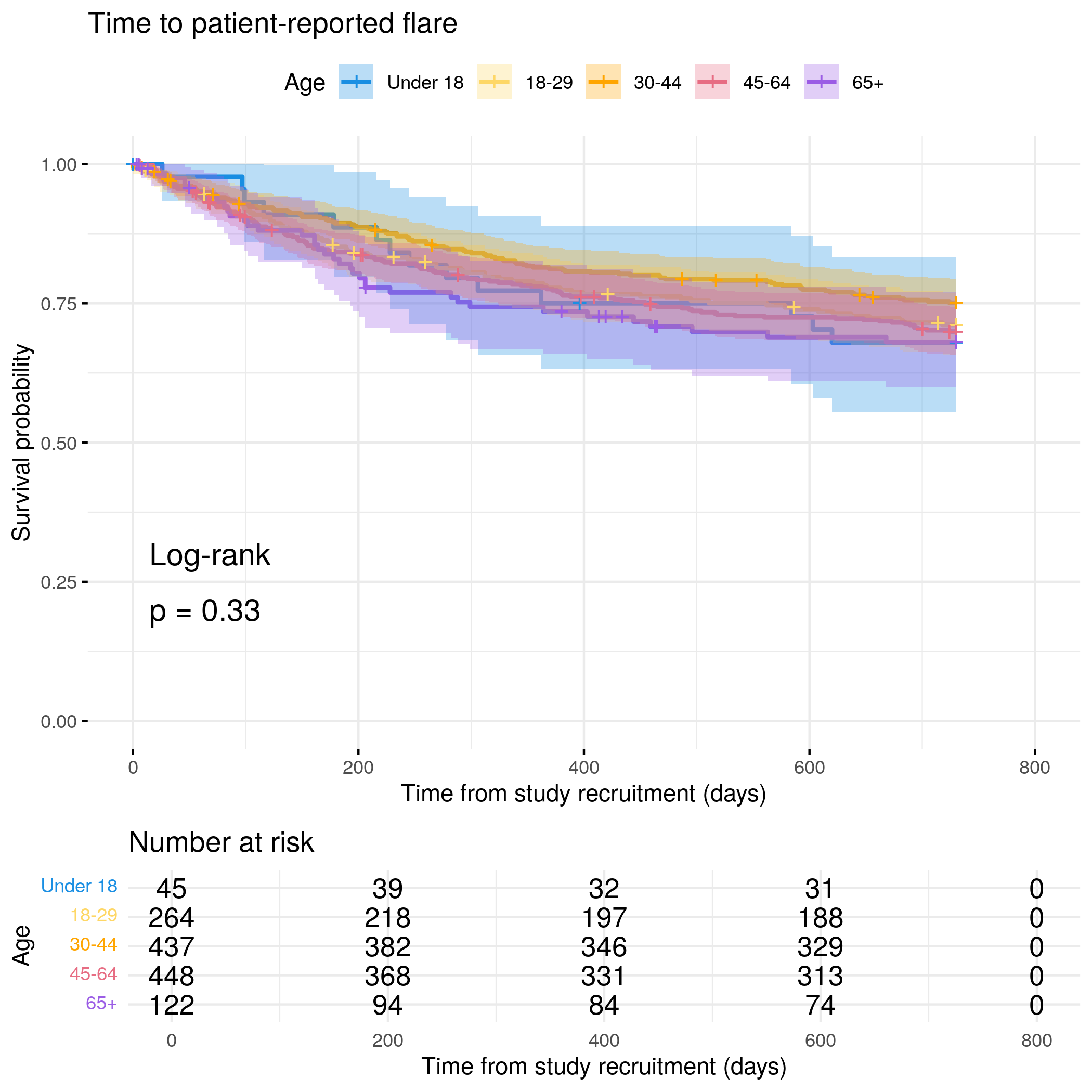
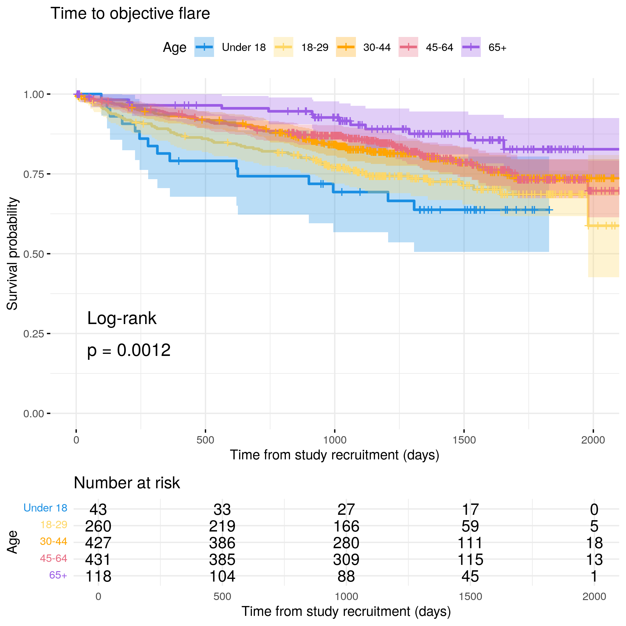
# Generate survival plot and run Cox model for objective flare
analysis_result <- run_survival_analysis(
  data = flare.cd.df,
  var_name = "Age",
  outcome_time = "hardflare_time",
  outcome_event = "hardflare",
  legend_title = "Age",
  plot_base_path = "plots/cd/hard-flare/demographics/age",
  break_time_by = 500
)

# Extract hazard ratio for Age (continuous variable)
fit.me <- coxph(
  Surv(hardflare_time, hardflare) ~ Sex + IMD + cat + Age + frailty(SiteNo),
  control = coxph.control(outer.max = 20),
  data = flare.cd.df
)

cd.hard.forest <- rbind(cd.hard.forest, get_HR(fit.me, "Age"))

# Display plot and model summary
knitr::include_graphics("plots/cd/hard-flare/demographics/age.png")

Code

invisible(cox_summary(fit.me, plot_base_path = "plots/cd/hard-flare/demographics/age"))

Cox model summary:

Variable	HR	Lower 95%	Upper 95%	P-value
SexFemale	1.4100	1.0742	1.8506	0.0133
IMD2	0.9220	0.5371	1.5828	0.7684
IMD3	0.9333	0.5377	1.6200	0.8061
IMD4	0.9037	0.5282	1.5462	0.7117
IMD5	0.9530	0.5672	1.6014	0.8559
catFC 50-250	2.0702	1.5083	2.8414	0.0000
catFC > 250	3.3191	2.3583	4.6712	0.0000
Age	0.9865	0.9779	0.9953	0.0026

Proportional hazards assumption test

	Chi-squared statistic	DF	P-value
Sex	0.2070	0.9856	0.6432
IMD	4.3372	3.9449	0.3546
cat	8.6873	1.9855	0.0128
Age	3.3245	0.9503	0.0635
GLOBAL	16.4294	18.2438	0.5790

`geom_smooth()` using formula = 'y ~ x'
`geom_smooth()` using formula = 'y ~ x'

[1] “plots/cd/hard-flare/demographics/age-dfbeta.png” attr(,“class”) [1] “knit_image_paths” “knit_asis”

`geom_smooth()` using formula = 'y ~ x'
`geom_smooth()` using formula = 'y ~ x'

[1] “plots/cd/hard-flare/demographics/age-martingale.png” attr(,“class”) [1] “knit_image_paths” “knit_asis”

Ulcerative colitis

Patient-reported flare
Objective flare

Code

# Categorize age
flare.uc.df <- categorize_variable(flare.uc.df, "Age", 
                                   breaks = c(0, 18, 30, 45, 65, Inf),
                                   labels = c("Under 18", "18-29", "30-44", "45-64", "65+"))

# Generate survival plot and run Cox model
analysis_result <- run_survival_analysis(
  data = flare.uc.df,
  var_name = "Age",
  outcome_time = "softflare_time",
  outcome_event = "softflare",
  legend_title = "Age",
  plot_base_path = "plots/uc/soft-flare/demographics/age",
  break_time_by = 200
)

# Extract hazard ratio for Age (continuous variable)
fit.me <- coxph(
  Surv(softflare_time, softflare) ~ Sex + IMD + cat + Age + frailty(SiteNo),
  control = coxph.control(outer.max = 20),
  data = flare.uc.df
)

uc.clin.forest <- rbind(uc.clin.forest, get_HR(fit.me, "Age"))

# Display plot and model summary
knitr::include_graphics("plots/uc/soft-flare/demographics/age.png")

Code

invisible(cox_summary(fit.me, plot_base_path = "plots/uc/soft-flare/demographics/age"))

Cox model summary:

Variable	HR	Lower 95%	Upper 95%	P-value
SexFemale	1.5135	1.2220	1.8747	0.0001
IMD2	1.2074	0.7621	1.9129	0.4220
IMD3	1.0923	0.6966	1.7126	0.7006
IMD4	1.4407	0.9378	2.2131	0.0955
IMD5	1.2134	0.7953	1.8512	0.3695
catFC 50-250	1.5856	1.2399	2.0277	0.0002
catFC > 250	2.1185	1.6228	2.7658	0.0000
Age	0.9928	0.9857	0.9998	0.0449

Proportional hazards assumption test

	Chi-squared statistic	DF	P-value
Sex	1.2765	0.9891	0.2555
IMD	3.9850	3.9439	0.3998
cat	5.7478	1.9712	0.0549
Age	0.2636	0.9656	0.5931
GLOBAL	11.8199	19.6624	0.9132

`geom_smooth()` using formula = 'y ~ x'
`geom_smooth()` using formula = 'y ~ x'

[1] “plots/uc/soft-flare/demographics/age-dfbeta.png” attr(,“class”) [1] “knit_image_paths” “knit_asis”

`geom_smooth()` using formula = 'y ~ x'
`geom_smooth()` using formula = 'y ~ x'

[1] “plots/uc/soft-flare/demographics/age-martingale.png” attr(,“class”) [1] “knit_image_paths” “knit_asis”

Code

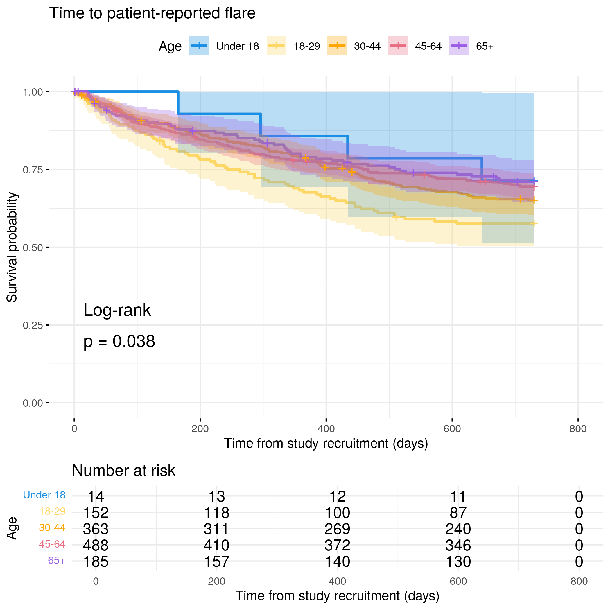
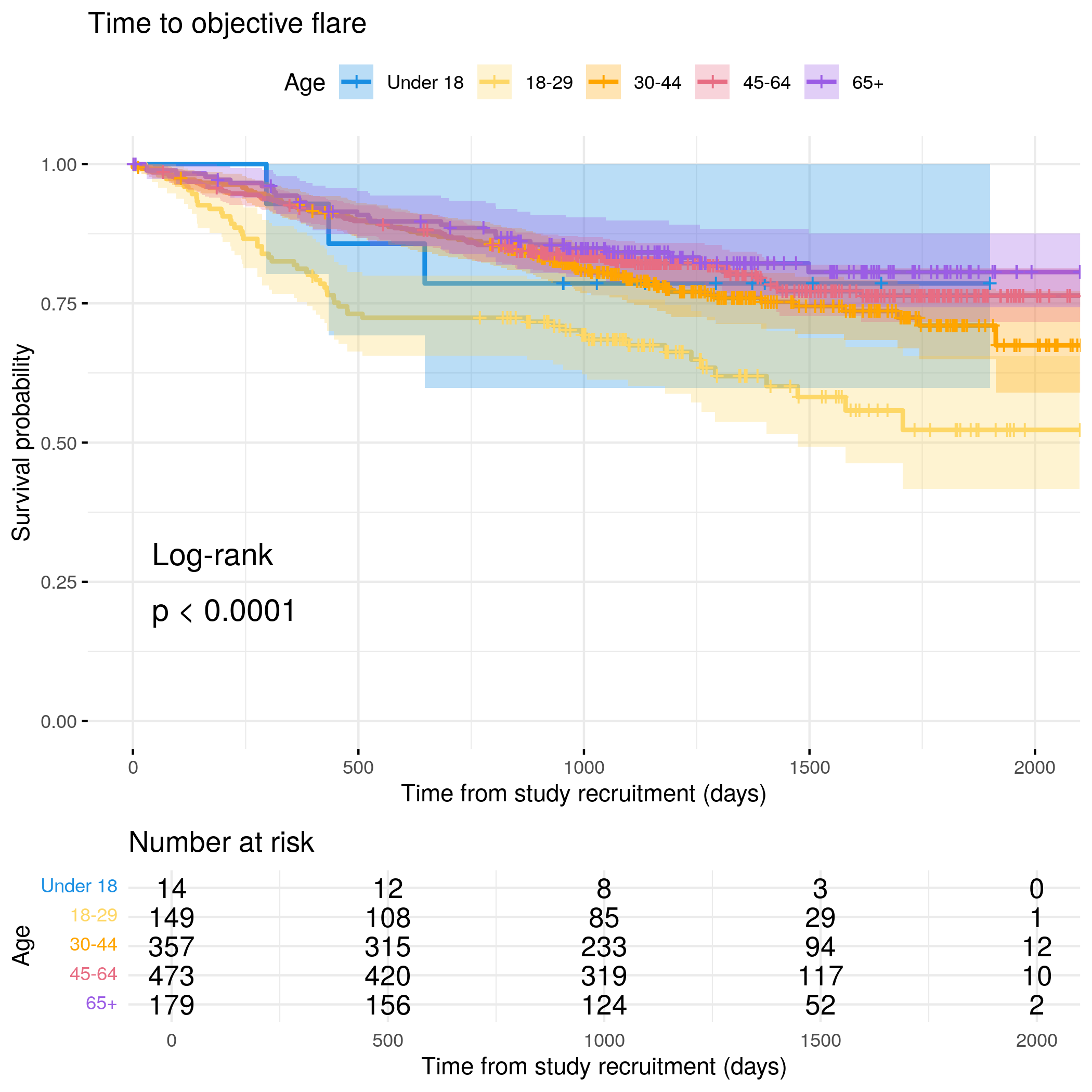
# Generate survival plot and run Cox model for objective flare
analysis_result <- run_survival_analysis(
  data = flare.uc.df,
  var_name = "Age",
  outcome_time = "hardflare_time",
  outcome_event = "hardflare",
  legend_title = "Age",
  plot_base_path = "plots/uc/hard-flare/demographics/age",
  break_time_by = 500
)

# Extract hazard ratio for Age (continuous variable)
fit.me <- coxph(
  Surv(hardflare_time, hardflare) ~ Sex + IMD + cat + Age + frailty(SiteNo),
  control = coxph.control(outer.max = 20),
  data = flare.uc.df
)

uc.hard.forest <- rbind(uc.hard.forest, get_HR(fit.me, "Age"))

# Display plot and model summary
knitr::include_graphics("plots/uc/hard-flare/demographics/age.png")

Code

invisible(cox_summary(fit.me, plot_base_path = "plots/uc/hard-flare/demographics/age"))

Cox model summary:

Variable	HR	Lower 95%	Upper 95%	P-value
SexFemale	1.2937	0.9958	1.6807	0.0538
IMD2	1.3555	0.7565	2.4289	0.3067
IMD3	1.3777	0.7842	2.4203	0.2650
IMD4	1.7536	1.0168	3.0242	0.0434
IMD5	1.3509	0.7875	2.3173	0.2747
catFC 50-250	2.0872	1.5288	2.8495	0.0000
catFC > 250	3.1867	2.3015	4.4124	0.0000
Age	0.9882	0.9794	0.9971	0.0094

Proportional hazards assumption test

	Chi-squared statistic	DF	P-value
Sex	0.1150	0.9847	0.7285
IMD	2.7089	3.9421	0.5986
cat	4.0990	1.9687	0.1255
Age	0.3529	0.9656	0.5381
GLOBAL	7.4819	23.1362	0.9991

`geom_smooth()` using formula = 'y ~ x'
`geom_smooth()` using formula = 'y ~ x'

[1] “plots/uc/hard-flare/demographics/age-dfbeta.png” attr(,“class”) [1] “knit_image_paths” “knit_asis”

`geom_smooth()` using formula = 'y ~ x'
`geom_smooth()` using formula = 'y ~ x'

[1] “plots/uc/hard-flare/demographics/age-martingale.png” attr(,“class”) [1] “knit_image_paths” “knit_asis”

BMI

Crohn’s disease

Patient-reported flare
Objective flare

Code

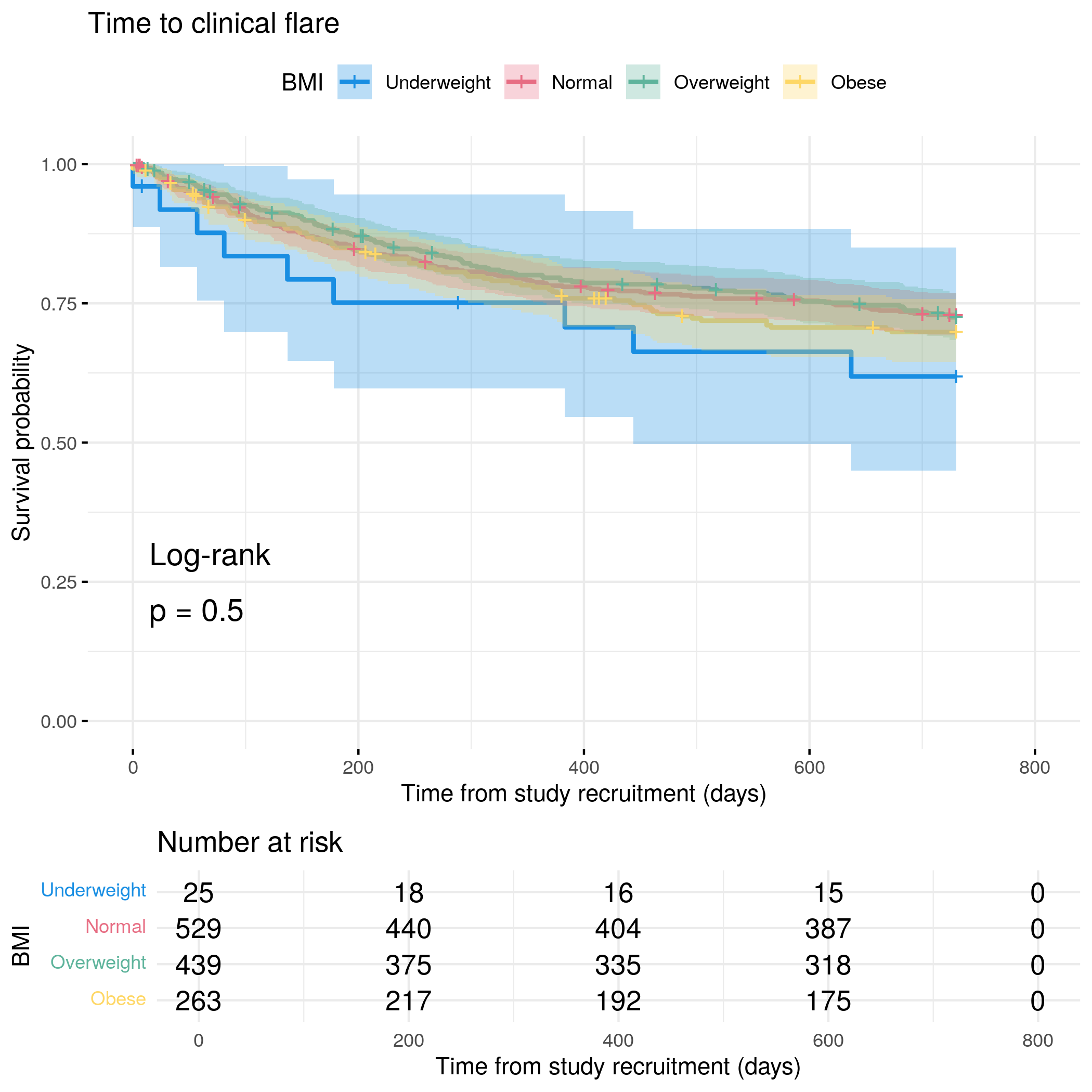
p <- generate_survival_plot(
  data = flare.cd.df,
  formula = Surv(softflare_time, softflare) ~ BMIcat,
  legend_title = "BMI",
  legend_labs = c("Underweight", "Normal", "Overweight", "Obese"),
  palette = c("#1A8FE3", "#E76D83", "#5FB49C", "#FED766"),
  xlab = "Time from study recruitment (days)",
  title = "Time to clinical flare",
  break_time_by = 200,
  plot_path = "plots/cd/soft-flare/demographics/bmi"
)

knitr::include_graphics("plots/cd/soft-flare/demographics/bmi.png")

Code

fit.me <- coxph(
  Surv(softflare_time, softflare) ~
    Sex + IMD + cat + BMI + frailty(SiteNo),
  control = coxph.control(outer.max = 20),
  data = flare.cd.df
)

cd.clin.forest <- rbind(
  cd.clin.forest,
  get_HR(fit.me, c("BMI"))
)

invisible(cox_summary(fit.me))

Cox model summary:

Variable	HR	Lower 95%	Upper 95%	P-value
SexFemale	2.1473	1.6736	2.7550	0.0000
IMD2	0.8998	0.5671	1.4279	0.6542
IMD3	0.8895	0.5555	1.4243	0.6258
IMD4	0.9343	0.5951	1.4667	0.7676
IMD5	0.9772	0.6332	1.5081	0.9171
catFC 50-250	1.5540	1.1972	2.0170	0.0009
catFC > 250	2.2569	1.6787	3.0342	0.0000
BMI	1.0122	0.9911	1.0337	0.2594

Proportional hazards assumption test

	Chi-squared statistic	DF	P-value
Sex	0.1734	0.9925	0.6740
IMD	6.5777	3.9477	0.1556
cat	1.5900	1.9797	0.4468
BMI	2.3144	0.9900	0.1265
GLOBAL	10.2401	14.8159	0.7941

`geom_smooth()` using formula = 'y ~ x'
`geom_smooth()` using formula = 'y ~ x'

Code

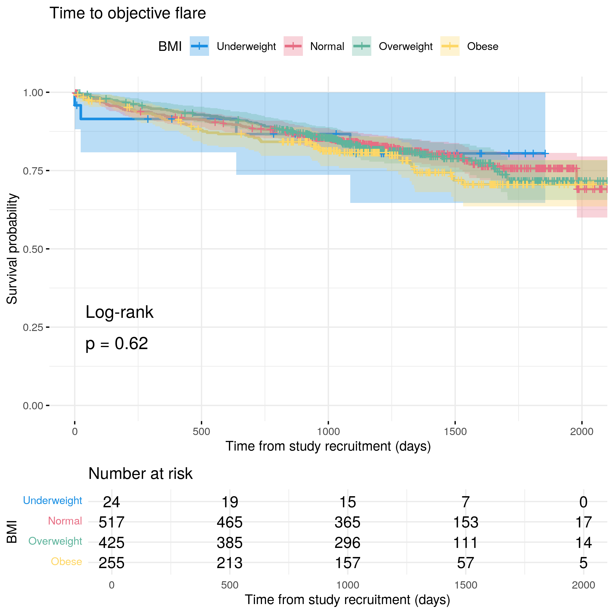
p <- generate_survival_plot(
  data = flare.cd.df,
  formula = Surv(hardflare_time, hardflare) ~ BMIcat,
  legend_title = "BMI",
  legend_labs = c("Underweight", "Normal", "Overweight", "Obese"),
  palette = c("#1A8FE3", "#E76D83", "#5FB49C", "#FED766"),
  xlab = "Time from study recruitment (days)",
  title = "Time to objective flare",
  break_time_by = 500,
  plot_path = "plots/cd/hard-flare/demographics/bmi"
)

knitr::include_graphics("plots/cd/hard-flare/demographics/bmi.png")

Code

fit.me <- coxph(
  Surv(hardflare_time, hardflare) ~
    Sex + IMD + cat + BMI + frailty(SiteNo),
  control = coxph.control(outer.max = 20),
  data = flare.cd.df
)

cd.hard.forest <- rbind(
  cd.hard.forest,
  get_HR(fit.me, c("BMI"))
)

invisible(cox_summary(fit.me))

Cox model summary:

Variable	HR	Lower 95%	Upper 95%	P-value
SexFemale	1.5011	1.1295	1.9950	0.0051
IMD2	0.9513	0.5451	1.6599	0.8604
IMD3	0.9658	0.5454	1.7103	0.9050
IMD4	0.8451	0.4830	1.4788	0.5556
IMD5	0.9334	0.5478	1.5906	0.8001
catFC 50-250	2.0103	1.4508	2.7857	0.0000
catFC > 250	3.1451	2.1945	4.5074	0.0000
BMI	1.0200	0.9949	1.0456	0.1187

Proportional hazards assumption test

	Chi-squared statistic	DF	P-value
Sex	0.8263	0.9880	0.3591
IMD	3.6654	3.9453	0.4448
cat	7.2453	1.9854	0.0263
BMI	3.8299	0.9886	0.0495
GLOBAL	15.1563	17.4781	0.6169

`geom_smooth()` using formula = 'y ~ x'
`geom_smooth()` using formula = 'y ~ x'

Ulcerative colitis

Patient-reported flare
Objective flare

Code

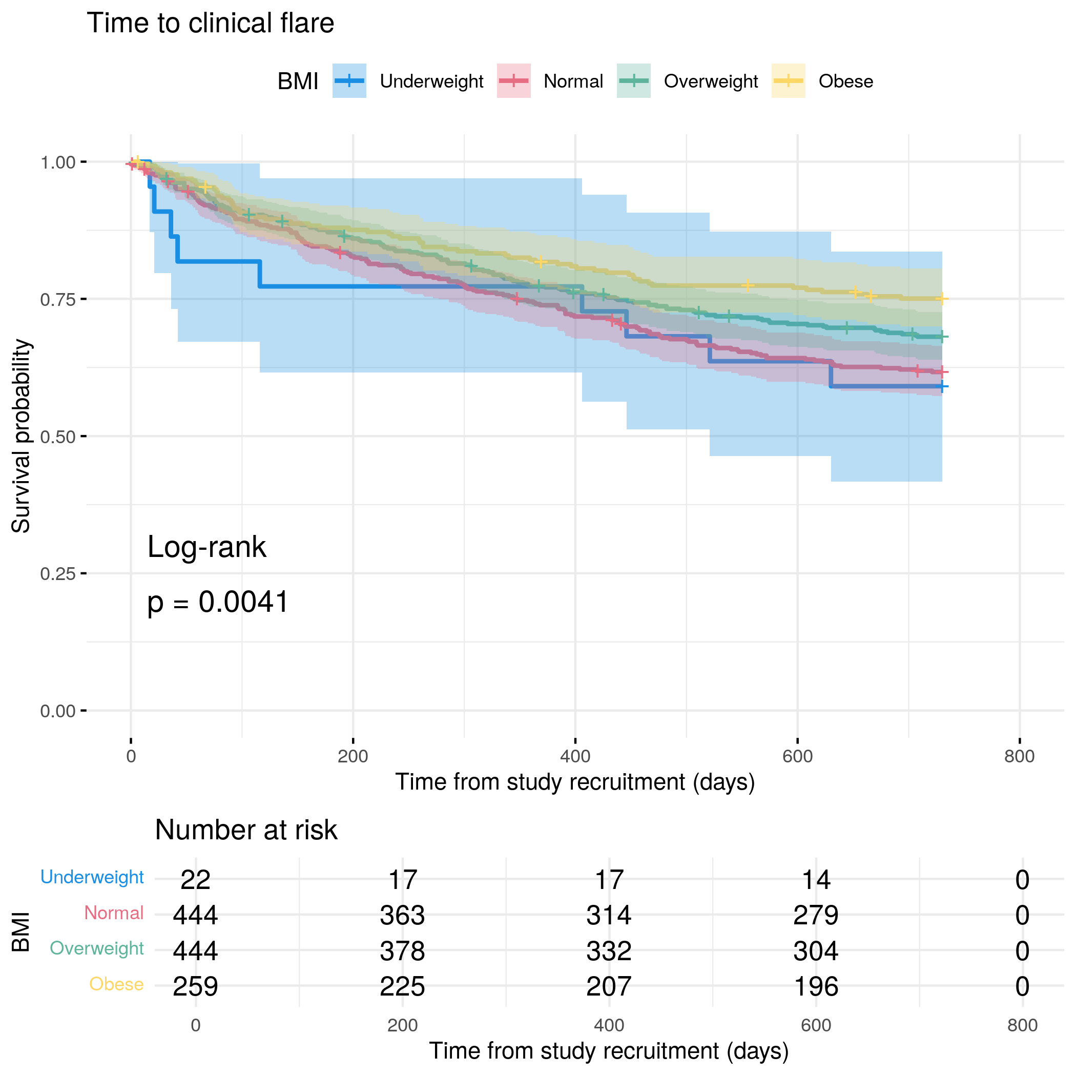
p <- generate_survival_plot(
  data = flare.uc.df,
  formula = Surv(softflare_time, softflare) ~ BMIcat,
  legend_title = "BMI",
  legend_labs = c("Underweight", "Normal", "Overweight", "Obese"),
  palette = c("#1A8FE3", "#E76D83", "#5FB49C", "#FED766"),
  xlab = "Time from study recruitment (days)",
  title = "Time to clinical flare",
  break_time_by = 200,
  plot_path = "plots/uc/soft-flare/demographics/bmi"
)

knitr::include_graphics("plots/uc/soft-flare/demographics/bmi.png")

Code

fit.me <- coxph(
  Surv(softflare_time, softflare) ~
    Sex + IMD + cat + BMI + frailty(SiteNo),
  control = coxph.control(outer.max = 20),
  data = flare.uc.df
)
uc.clin.forest <- rbind(
  uc.clin.forest,
  get_HR(fit.me, c("BMI"))
)
invisible(cox_summary(fit.me))

Cox model summary:

Variable	HR	Lower 95%	Upper 95%	P-value
SexFemale	1.5667	1.2601	1.9478	0.0001
IMD2	1.2357	0.7747	1.9711	0.3743
IMD3	1.0037	0.6340	1.5890	0.9873
IMD4	1.4156	0.9159	2.1878	0.1177
IMD5	1.1137	0.7241	1.7128	0.6240
catFC 50-250	1.6181	1.2586	2.0803	0.0002
catFC > 250	2.1566	1.6473	2.8235	0.0000
BMI	0.9686	0.9481	0.9896	0.0035

Proportional hazards assumption test

	Chi-squared statistic	DF	P-value
Sex	1.3437	0.9904	0.2438
IMD	3.8474	3.9456	0.4189
cat	4.7128	1.9726	0.0925
BMI	0.4838	0.9851	0.4807
GLOBAL	10.4559	17.3504	0.8958

`geom_smooth()` using formula = 'y ~ x'
`geom_smooth()` using formula = 'y ~ x'

Code

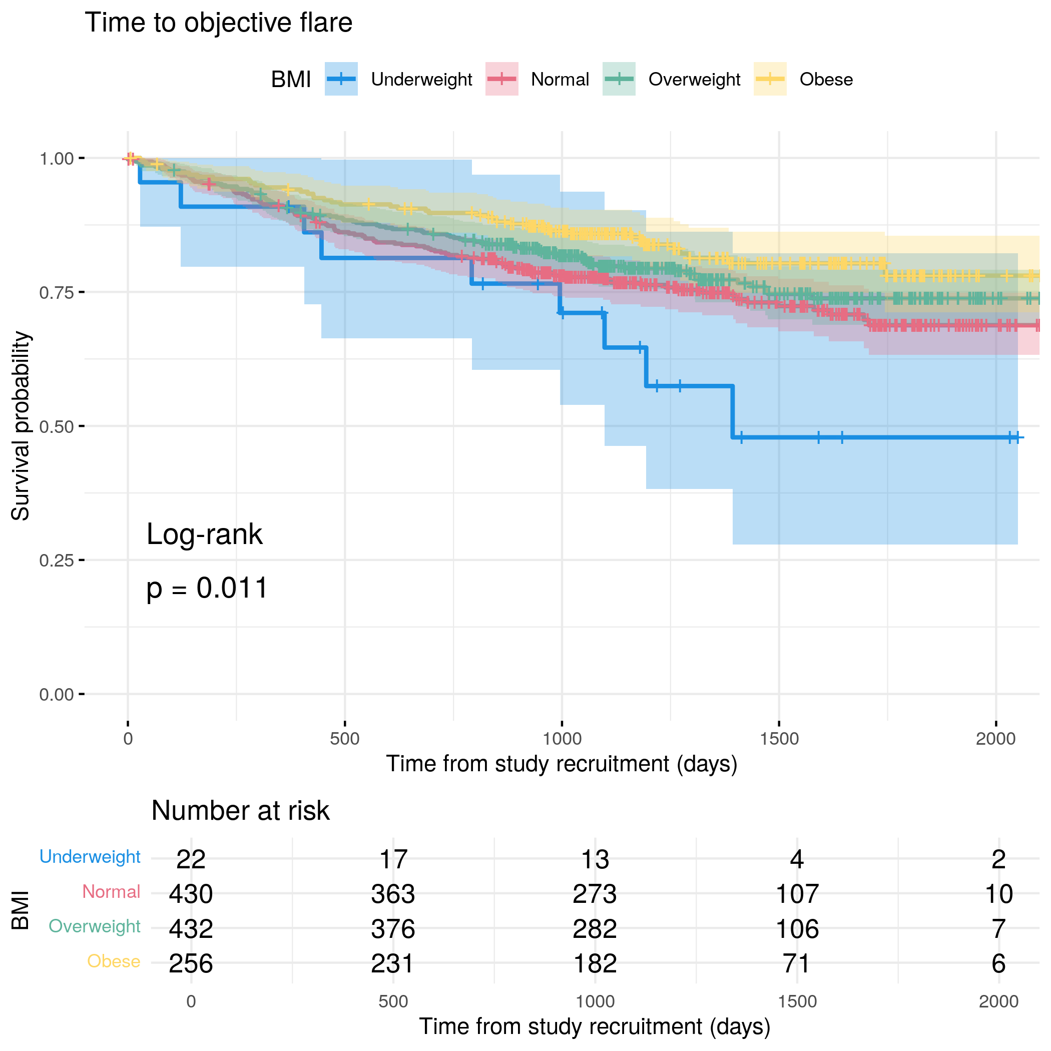
p <- generate_survival_plot(
  data = flare.uc.df,
  formula = Surv(hardflare_time, hardflare) ~ BMIcat,
  legend_title = "BMI",
  legend_labs = c("Underweight", "Normal", "Overweight", "Obese"),
  palette = c("#1A8FE3", "#E76D83", "#5FB49C", "#FED766"),
  xlab = "Time from study recruitment (days)",
  title = "Time to objective flare",
  break_time_by = 500,
  plot_path = "plots/uc/hard-flare/demographics/bmi"
)

knitr::include_graphics("plots/uc/hard-flare/demographics/bmi.png")

Code

fit.me <- coxph(
  Surv(hardflare_time, hardflare) ~
    Sex + IMD + cat + BMI + frailty(SiteNo),
  control = coxph.control(outer.max = 20),
  data = flare.uc.df
)
uc.hard.forest <- rbind(
  uc.hard.forest,
  get_HR(fit.me, "BMI")
  )
invisible(cox_summary(fit.me))

Cox model summary:

Variable	HR	Lower 95%	Upper 95%	P-value
SexFemale	1.3542	1.0359	1.7703	0.0265
IMD2	1.4226	0.7804	2.5931	0.2499
IMD3	1.3567	0.7598	2.4225	0.3024
IMD4	1.7491	0.9986	3.0636	0.0506
IMD5	1.2764	0.7316	2.2270	0.3902
catFC 50-250	2.0568	1.4948	2.8299	0.0000
catFC > 250	3.2137	2.3058	4.4790	0.0000
BMI	0.9808	0.9558	1.0065	0.1415

Proportional hazards assumption test

	Chi-squared statistic	DF	P-value
Sex	0.1486	0.9850	0.6938
IMD	2.5015	3.9358	0.6345
cat	3.5648	1.9672	0.1640
BMI	0.1512	0.9853	0.6915
GLOBAL	6.9035	22.4944	0.9993

`geom_smooth()` using formula = 'y ~ x'
`geom_smooth()` using formula = 'y ~ x'

Code

saveRDS(flare.df, paste0(paths$outdir, "flares-demographics.RDS"))
saveRDS(flare.cd.df, paste0(paths$outdir, "flares-demographics-cd.RDS"))
saveRDS(flare.uc.df, paste0(paths$outdir, "flares-demographics-uc.RDS"))

saveRDS(cd.clin.forest, paste0(paths$outdir, "cd-clin-demographics.RDS"))
saveRDS(cd.hard.forest, paste0(paths$outdir, "cd-hard-demographics.RDS"))
saveRDS(uc.clin.forest, paste0(paths$outdir, "uc-clin-demographics.RDS"))
saveRDS(uc.hard.forest, paste0(paths$outdir, "uc-hard-demographics.RDS"))

Control for additional covariates

Crohn’s disease

Patient-reported flare

Code

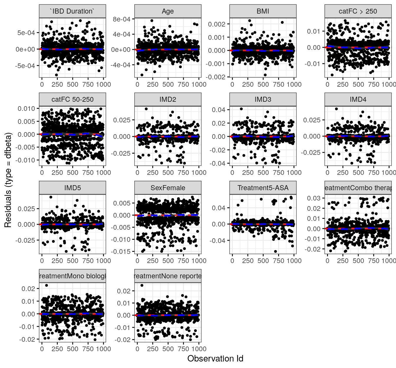
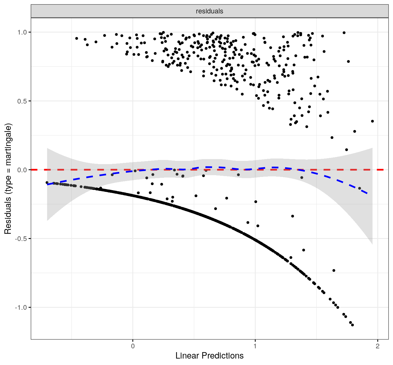
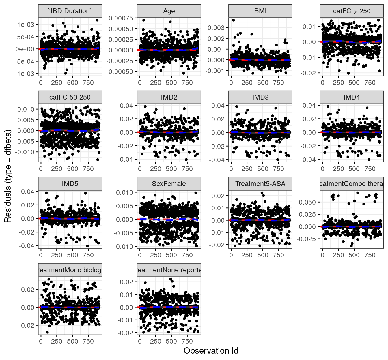
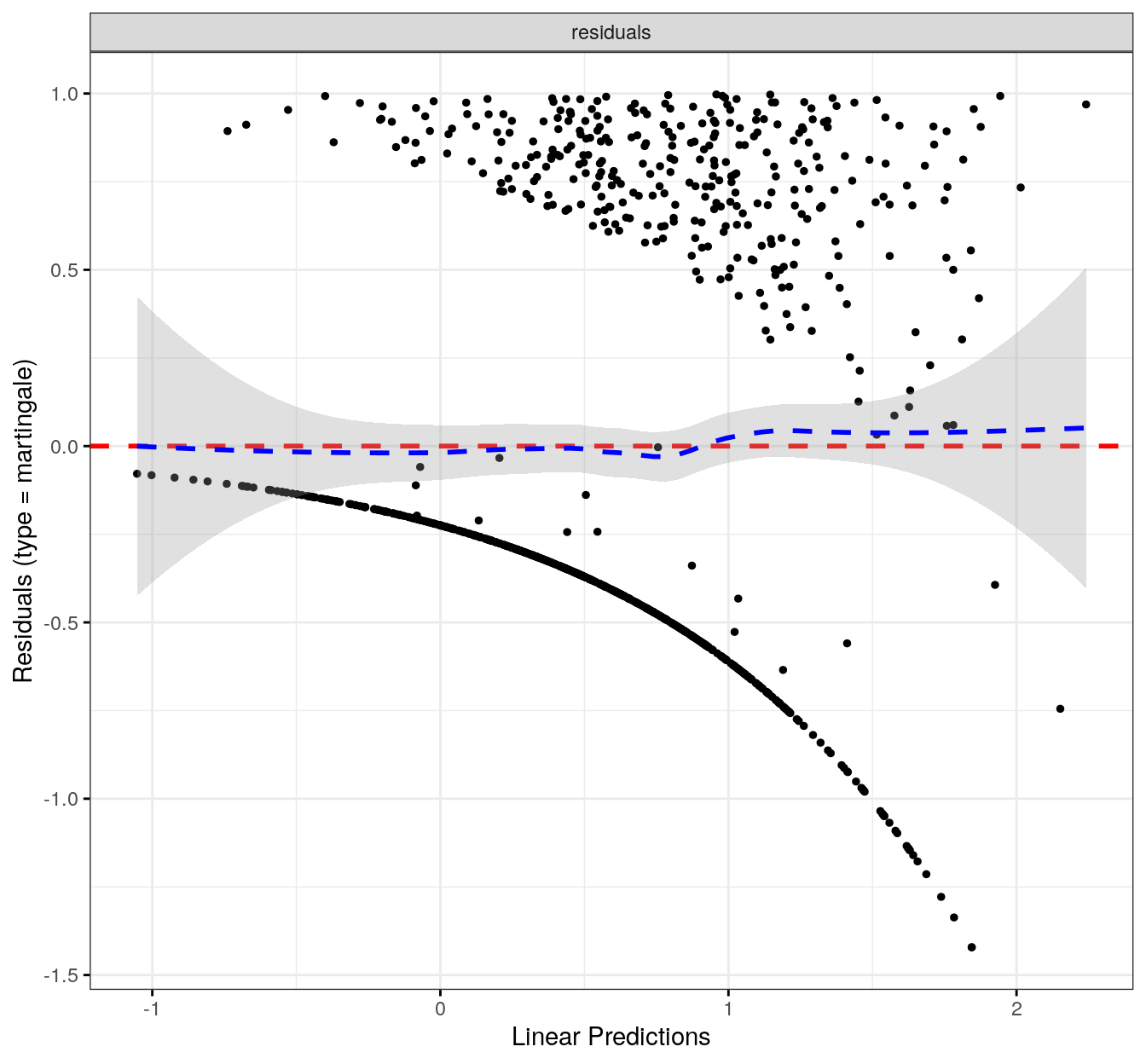
fit.me <- coxph(
  Surv(softflare_time, softflare) ~
    Sex +
    IMD +
    cat + 
    `IBD Duration` +
    BMI +
    Treatment +
    Age +
    frailty(SiteNo),
  control = coxph.control(outer.max = 20),
  data = flare.cd.df
)

invisible(cox_summary(fit.me))

Cox model summary:

Variable	HR	Lower 95%	Upper 95%	P-value
SexFemale	2.1585	1.6671	2.7947	0.0000
IMD2	0.8389	0.5280	1.3326	0.4569
IMD3	0.8199	0.5074	1.3247	0.4172
IMD4	0.8984	0.5702	1.4156	0.6442
IMD5	0.9268	0.5991	1.4337	0.7327
catFC 50-250	1.4944	1.1441	1.9521	0.0032
catFC > 250	2.1836	1.6127	2.9566	0.0000
`IBD Duration`	0.9942	0.9829	1.0056	0.3152
BMI	1.0040	0.9821	1.0264	0.7231
TreatmentMono biologic	0.9820	0.6903	1.3971	0.9197
TreatmentCombo therapy	0.7083	0.4599	1.0909	0.1175
Treatment5-ASA	1.3322	0.7502	2.3657	0.3276
TreatmentNone reported	0.9726	0.7007	1.3502	0.8683
Age	1.0046	0.9957	1.0136	0.3112

Proportional hazards assumption test

	Chi-squared statistic	DF	P-value
Sex	0.4811	0.9924	0.4849
IMD	5.6223	3.9577	0.2246
cat	1.4933	1.9842	0.4702
`IBD Duration`	3.5316	0.9957	0.0598
BMI	2.1568	0.9913	0.1404
Treatment	3.4530	3.9163	0.4721
Age	2.1438	0.9913	0.1416
GLOBAL	18.1663	18.5875	0.4840

`geom_smooth()` using formula = 'y ~ x'

`geom_smooth()` using formula = 'y ~ x'

Objective flare

Code

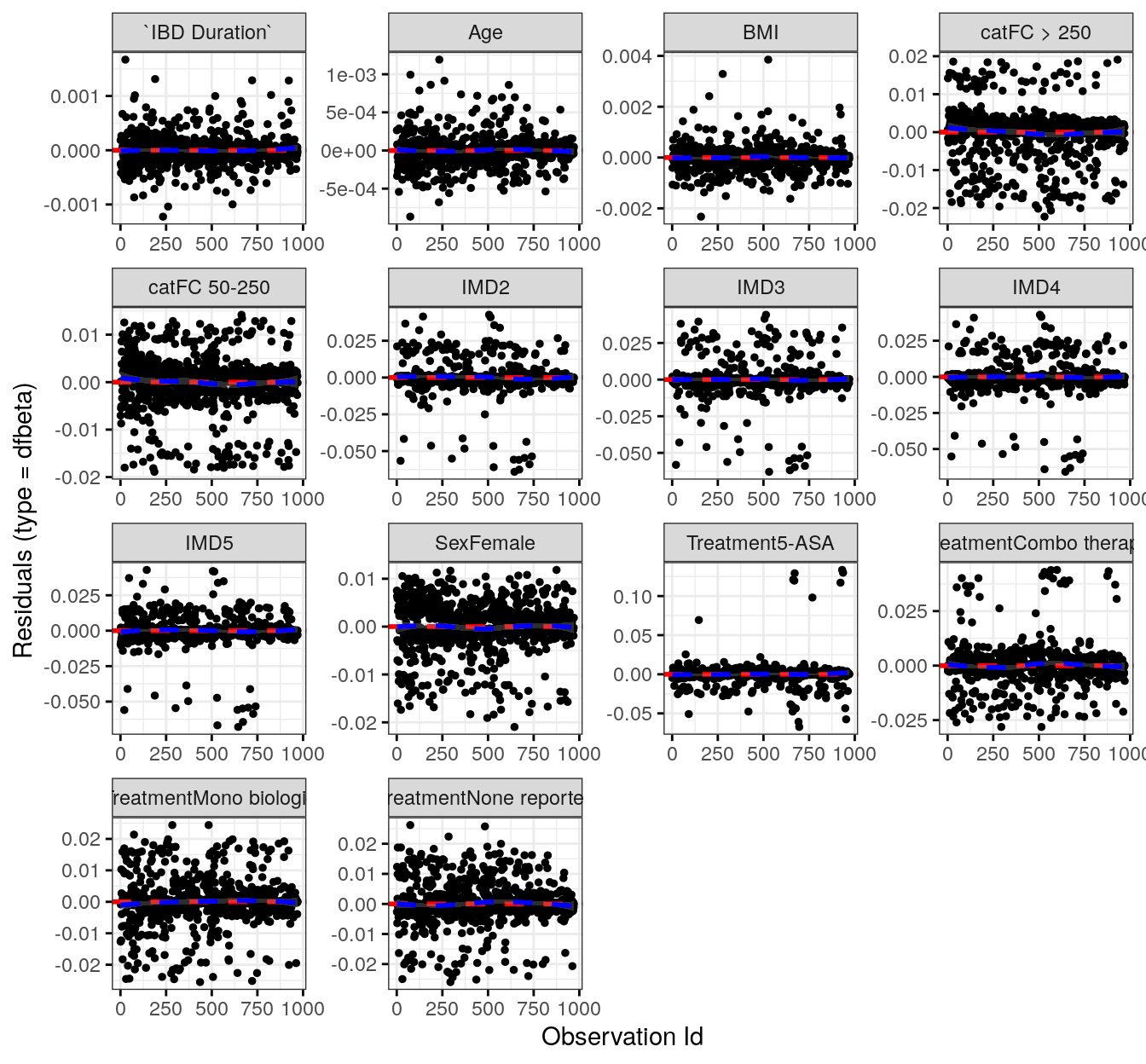
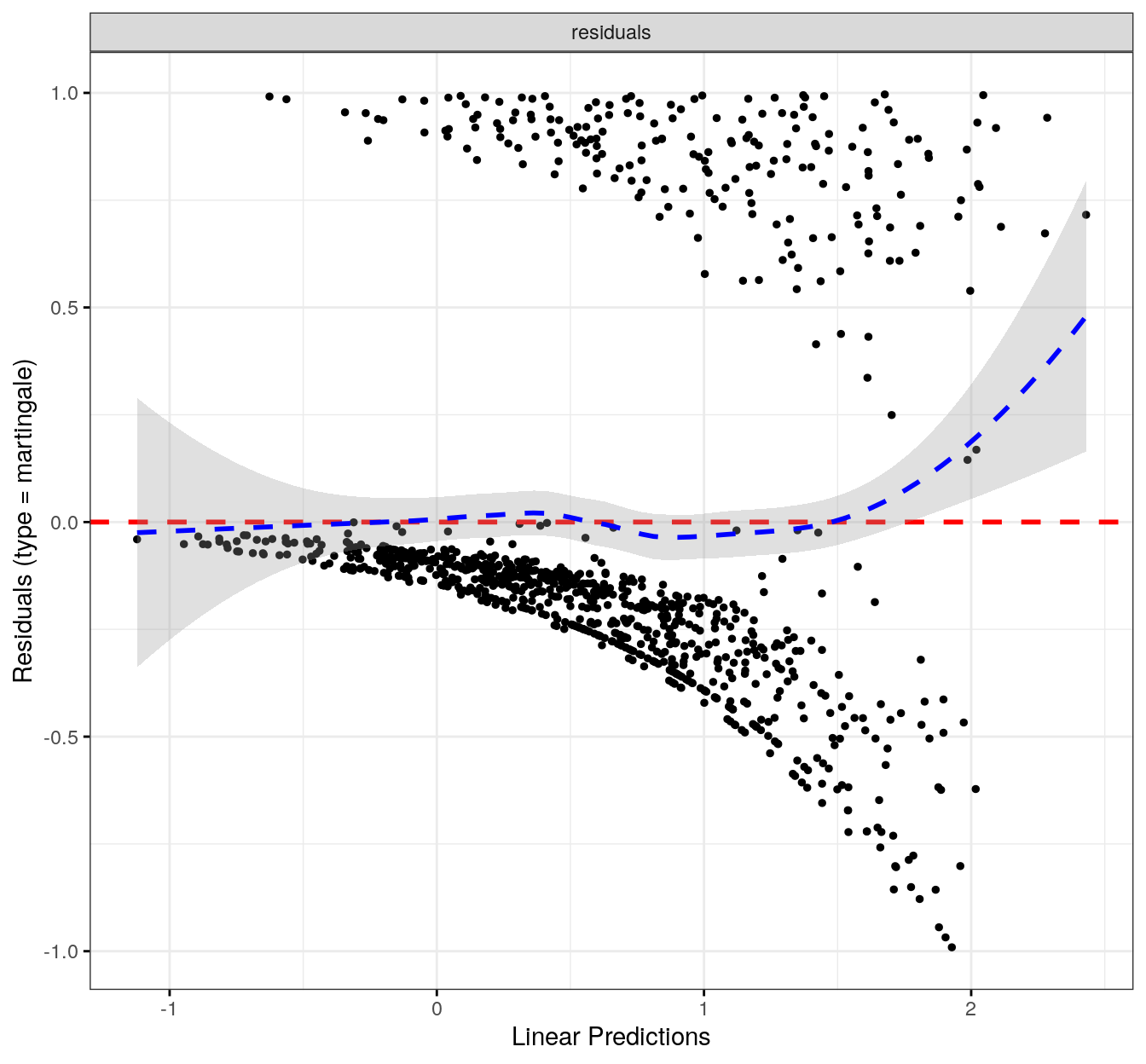
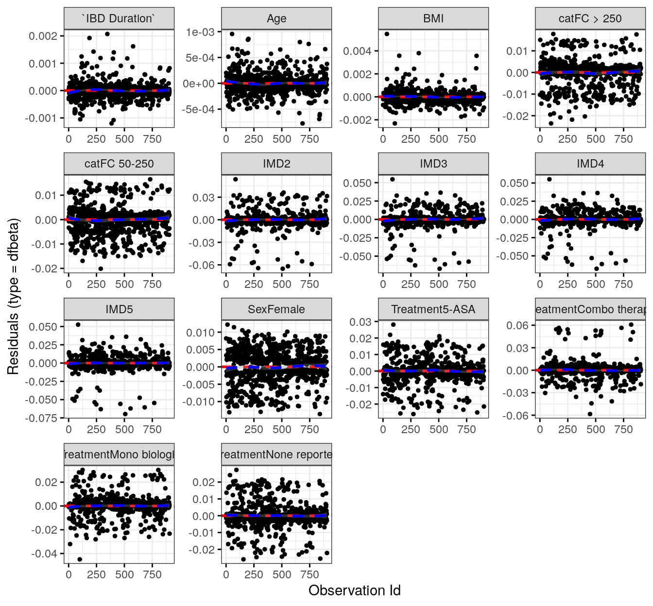
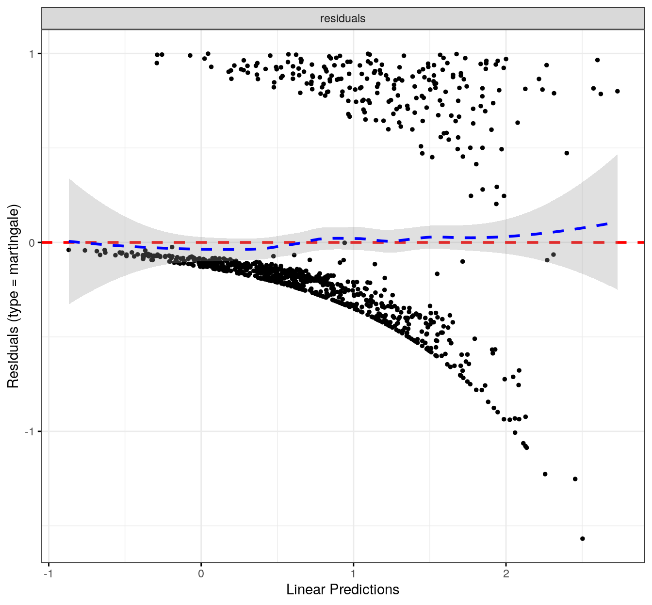
fit.me <- coxph(
  Surv(hardflare_time, hardflare) ~
    Sex +
    IMD +
    cat +
    `IBD Duration` +
    BMI +
    Treatment + 
    Age +
    frailty(SiteNo),
  control = coxph.control(outer.max = 20),
  data = flare.cd.df
)

invisible(cox_summary(fit.me))

Cox model summary:

Variable	HR	Lower 95%	Upper 95%	P-value
SexFemale	1.7096	1.2650	2.3103	0.0005
IMD2	0.9875	0.5574	1.7494	0.9656
IMD3	0.8917	0.4907	1.6203	0.7068
IMD4	0.9573	0.5384	1.7022	0.8819
IMD5	1.0963	0.6346	1.8936	0.7417
catFC 50-250	2.0382	1.4550	2.8550	0.0000
catFC > 250	3.2590	2.2523	4.7158	0.0000
`IBD Duration`	0.9861	0.9714	1.0009	0.0659
BMI	1.0172	0.9912	1.0439	0.1964
TreatmentMono biologic	0.9700	0.6482	1.4516	0.8824
TreatmentCombo therapy	0.6422	0.3867	1.0667	0.0872
Treatment5-ASA	1.2541	0.5732	2.7438	0.5708
TreatmentNone reported	0.7334	0.4971	1.0822	0.1183
Age	0.9883	0.9777	0.9991	0.0331

Proportional hazards assumption test

	Chi-squared statistic	DF	P-value
Sex	0.3823	0.9866	0.5308
IMD	2.0716	3.9513	0.7157
cat	7.1574	1.9870	0.0275
`IBD Duration`	0.1161	0.9959	0.7317
BMI	4.6695	0.9901	0.0302
Treatment	3.4118	3.8994	0.4757
Age	4.6542	0.9917	0.0306
GLOBAL	21.4207	20.1145	0.3796

`geom_smooth()` using formula = 'y ~ x'

`geom_smooth()` using formula = 'y ~ x'

Ulcerative colitis

Proportional hazards assumption test
Proportional hazards assumption test

	Chi-squared statistic	DF	P-value
Sex	2.0073	0.9894	0.1545
IMD	2.7380	3.9498	0.5947
cat	4.7086	1.9739	0.0928
`IBD Duration`	1.4602	0.9878	0.2238
BMI	0.8736	0.9870	0.3455
Treatment	6.8299	3.8847	0.1362
Age	0.0002	0.9708	0.9859
GLOBAL	19.3518	22.4353	0.6489

`geom_smooth()` using formula = 'y ~ x'

`geom_smooth()` using formula = 'y ~ x'

Objective flare

Code

fit.me <- coxph( 
  Surv(hardflare_time, hardflare) ~
    Sex +
    IMD +
    cat +
    `IBD Duration` +
    BMI +
    Treatment +
    Age +
    frailty(SiteNo),
  control = coxph.control(outer.max = 20),
  data = flare.uc.df
)

invisible(cox_summary(fit.me))

Cox model summary:

Variable	HR	Lower 95%	Upper 95%	P-value
SexFemale	1.3830	1.0513	1.8193	0.0205
IMD2	1.3785	0.7491	2.5367	0.3023
IMD3	1.3342	0.7445	2.3909	0.3328
IMD4	1.7384	0.9880	3.0586	0.0551
IMD5	1.3577	0.7709	2.3911	0.2897
catFC 50-250	2.0810	1.5031	2.8811	0.0000
catFC > 250	3.1245	2.2284	4.3809	0.0000
`IBD Duration`	0.9925	0.9768	1.0085	0.3577
BMI	0.9851	0.9586	1.0123	0.2790
TreatmentMono biologic	1.1017	0.6979	1.7389	0.6776
TreatmentCombo therapy	0.9240	0.5166	1.6527	0.7899
Treatment5-ASA	0.9166	0.6162	1.3634	0.6672
TreatmentNone reported	0.7616	0.5073	1.1434	0.1890
Age	0.9903	0.9796	1.0010	0.0753

	Chi-squared statistic	DF	P-value
Sex	0.1289	0.9853	0.7137
IMD	1.2073	3.9393	0.8712
cat	4.0138	1.9712	0.1313
`IBD Duration`	0.4354	0.9841	0.5028
BMI	0.0764	0.9848	0.7767
Treatment	22.5860	3.8453	0.0001
Age	0.9837	0.9722	0.3122
GLOBAL	31.5988	25.2734	0.1796

`geom_smooth()` using formula = 'y ~ x'

`geom_smooth()` using formula = 'y ~ x'

Reproduction and reproducibility

Session info

R version 4.4.0 (2024-04-24)

Platform: aarch64-unknown-linux-gnu

locale: LC_CTYPE=en_US.UTF-8, LC_NUMERIC=C, LC_TIME=en_US.UTF-8, LC_COLLATE=en_US.UTF-8, LC_MONETARY=en_US.UTF-8, LC_MESSAGES=en_US.UTF-8, LC_PAPER=en_US.UTF-8, LC_NAME=C, LC_ADDRESS=C, LC_TELEPHONE=C, LC_MEASUREMENT=en_US.UTF-8 and LC_IDENTIFICATION=C

attached base packages: grid, stats, graphics, grDevices, utils, datasets, methods and base

other attached packages: gtsummary(v.1.7.2), DescTools(v.0.99.54), finalfit(v.1.0.7), coxme(v.2.2-20), bdsmatrix(v.1.3-7), pander(v.0.6.5), survminer(v.0.4.9), ggpubr(v.0.6.0), survival(v.3.5-8), datefixR(v.1.6.1), lubridate(v.1.9.3), forcats(v.1.0.0), stringr(v.1.5.1), dplyr(v.1.1.4), purrr(v.1.0.2), readr(v.2.1.5), tidyr(v.1.3.1), tibble(v.3.2.1), ggplot2(v.3.5.1), tidyverse(v.2.0.0), readxl(v.1.4.3), forestplot(v.3.1.6), abind(v.1.4-5) and checkmate(v.2.3.2)

loaded via a namespace (and not attached): gridExtra(v.2.3), gld(v.2.6.6), rlang(v.1.1.3), magrittr(v.2.0.3), e1071(v.1.7-14), compiler(v.4.4.0), mgcv(v.1.9-1), systemfonts(v.1.3.1), vctrs(v.0.6.5), pkgconfig(v.2.0.3), shape(v.1.4.6.1), fastmap(v.1.2.0), backports(v.1.5.0), labeling(v.0.4.3), KMsurv(v.0.1-5), utf8(v.1.2.4), rmarkdown(v.2.27), markdown(v.1.12), tzdb(v.0.4.0), nloptr(v.2.0.3), ragg(v.1.3.2), xfun(v.0.44), glmnet(v.4.1-8), jomo(v.2.7-6), jsonlite(v.1.8.8), pan(v.1.9), broom(v.1.0.6), R6(v.2.5.1), stringi(v.1.8.4), car(v.3.1-2), boot(v.1.3-30), rpart(v.4.1.23), cellranger(v.1.1.0), Rcpp(v.1.0.12), iterators(v.1.0.14), knitr(v.1.47), zoo(v.1.8-12), Matrix(v.1.7-0), splines(v.4.4.0), nnet(v.7.3-19), timechange(v.0.3.0), tidyselect(v.1.2.1), rstudioapi(v.0.16.0), yaml(v.2.3.8), ggtext(v.0.1.2), codetools(v.0.2-20), lattice(v.0.22-6), withr(v.3.0.0), evaluate(v.0.23), proxy(v.0.4-27), xml2(v.1.3.6), survMisc(v.0.5.6), pillar(v.1.9.0), carData(v.3.0-5), mice(v.3.16.0), foreach(v.1.5.2), generics(v.0.1.3), hms(v.1.1.3), commonmark(v.1.9.1), munsell(v.0.5.1), scales(v.1.3.0), rootSolve(v.1.8.2.4), minqa(v.1.2.7), xtable(v.1.8-4), class(v.7.3-22), glue(v.1.7.0), lmom(v.3.0), tools(v.4.4.0), data.table(v.1.15.4), lme4(v.1.1-35.3), ggsignif(v.0.6.4), Exact(v.3.2), mvtnorm(v.1.2-5), colorspace(v.2.1-0), nlme(v.3.1-164), cli(v.3.6.2), km.ci(v.0.5-6), textshaping(v.0.4.0), fansi(v.1.0.6), expm(v.0.999-9), broom.helpers(v.1.15.0), gt(v.0.10.1), gtable(v.0.3.5), rstatix(v.0.7.2), digest(v.0.6.35), farver(v.2.1.2), htmlwidgets(v.1.6.4), htmltools(v.0.5.8.1), lifecycle(v.1.0.4), httr(v.1.4.7), mitml(v.0.4-5), gridtext(v.0.1.5) and MASS(v.7.3-60.2)

Licensed by CC BY unless otherwise stated.